7 Null simulation results
We performed bootstrap-based and synthetic simulation analyses to evaluate the estimation of the distribution of TF under the global null hypothesis (equation Ref XX).
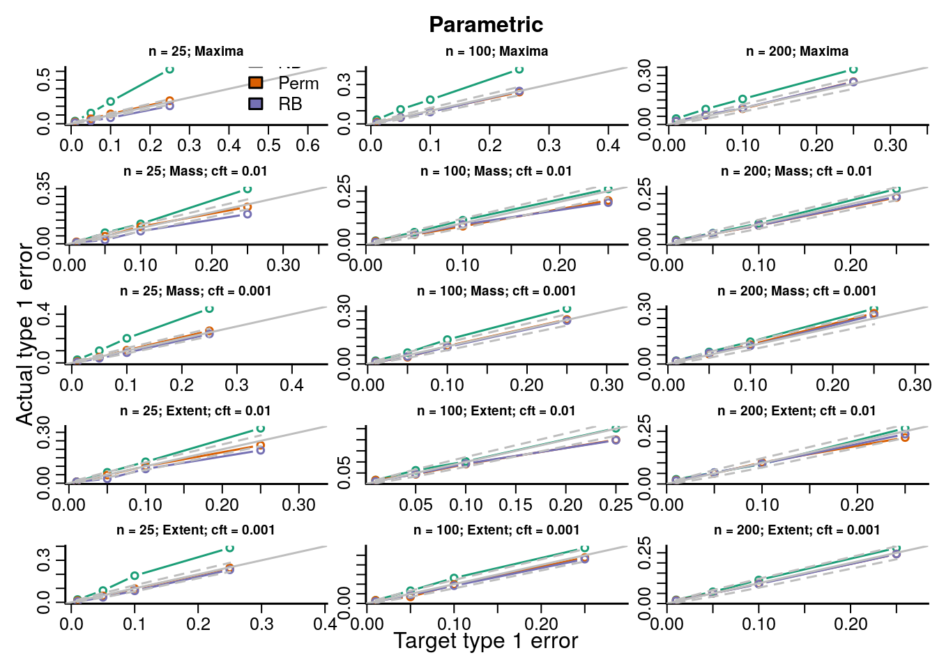
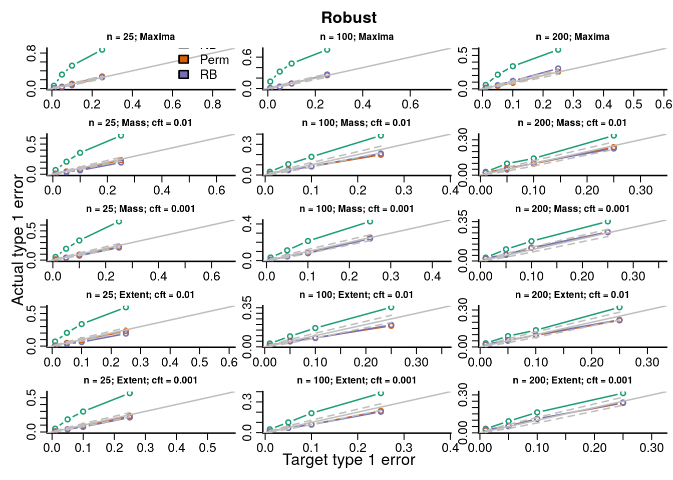
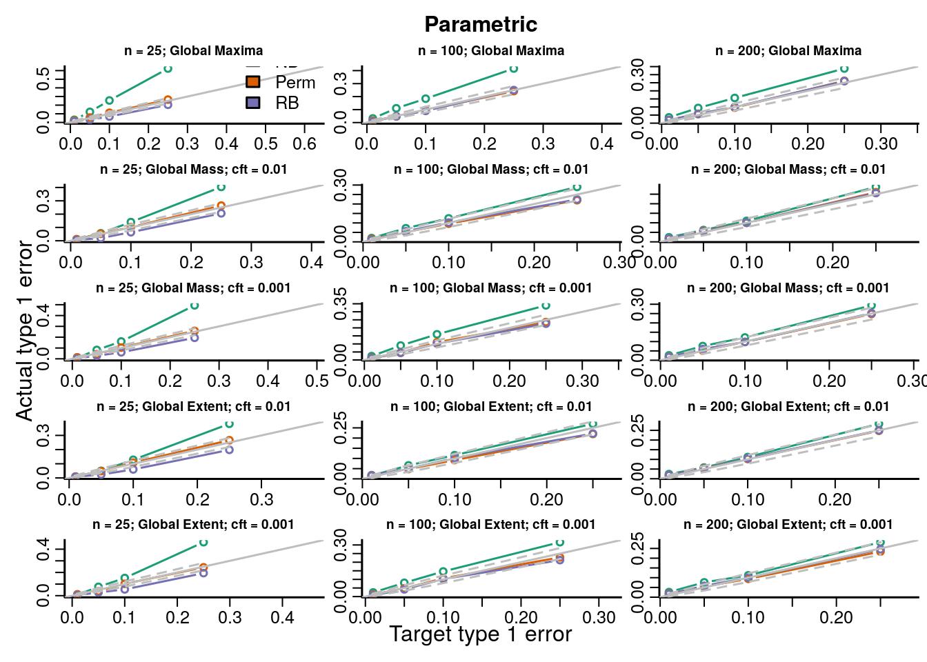
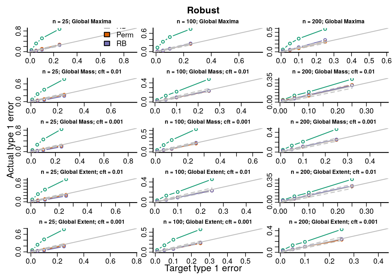
The type 1 error rates compare the proportion of datasets across all simulations with \(p\)-values less than the target type 1 error rate and show how accurate each procedure is for hypothesis testing. If the points fall on the identity line then the procedure maintains the type 1 error rate at the nominal level; below the line is conservative, and above the line is anticonservative.
The QQ plots compare the quantiles of the bootstrap distributions to the quantiles of the simulated distribution. Each line represents one simulated data set. The x-axis the the resampled estimates of the quantiles and the y-axis is the quantiles across the simulations, shown for \(q\in\)XX. This plot shows how good each procedure is at estimating the distribution of the TF (under the null) and the variability of the estimate across data sets. The best procedure will fall on the identity line and have a tight clustering around the line.
7.1 Synthetic null simulations
We simulated data under known heteroskedasticity to evaluate how the different resampling inference procedures perform in reproducing the distributions of TFs under the null. All resampling methods had near nominal type 1 error rates under homoskedasticity for parametric and robust test statistics, with the permutation and Rademacher bootstrap methods having slightly better accuracy than the normal bootstrap ({}). Under heteroskedasticity the permutation procedure had inflated error rates for parametric statistics, but not for robust test statistics. The two bootstrap methods had near nominal type 1 error rates. Simply using a robust covariance estimator resolves the problem with the permutation inference procedure because the procedure is scaling out the differences in the variances across subjects in each permutation by computing the square root covariance matrix as a function of the permuted data \(\eqref{eq:permutationSampleExchangeability}\).
7.2 Bootstrap null simulations using a factor covariate
In order to evaluate the type 1 error rate when performing an F-test of a factor covariate we simulated group independently of the imaging data and the bootstrap samples of the imaging data were modeled and tested on 3 degrees of freedom (4 groups). We evaluate parametric and robust test statistics and marginal and global null distributions as described in Section XX and Table XX. Type 1 error rates and QQ-plots are shown below. We gave a description of how to interpret the plots above in Section XX.
7.2.1 Marginal distribution
## Warning in FUN(X[[i]], ...): no non-missing arguments to max; returning -Inf

## Warning in FUN(X[[i]], ...): no non-missing arguments to max; returning -Inf
## MaximaMass; cft = 0.01Mass; cft = 0.001Extent; cft = 0.01Extent; cft = 0.001Global MaximaGlobal Mass; cft = 0.01Global Mass; cft = 0.001Global Extent; cft = 0.01Global Extent; cft = 0.001## Warning in FUN(X[[i]], ...): no non-missing arguments to max; returning -Inf
## Warning in FUN(X[[i]], ...): no non-missing arguments to max; returning -Inf## MaximaMass; cft = 0.01Mass; cft = 0.001Extent; cft = 0.01Extent; cft = 0.001Global MaximaGlobal Mass; cft = 0.01Global Mass; cft = 0.001Global Extent; cft = 0.01Global Extent; cft = 0.001## Warning in FUN(X[[i]], ...): no non-missing arguments to max; returning -Inf
## Warning in FUN(X[[i]], ...): no non-missing arguments to max; returning -Inf## MaximaMass; cft = 0.01Mass; cft = 0.001Extent; cft = 0.01Extent; cft = 0.001Global MaximaGlobal Mass; cft = 0.01Global Mass; cft = 0.001Global Extent; cft = 0.01Global Extent; cft = 0.001## Warning in FUN(X[[i]], ...): no non-missing arguments to max; returning -Inf
## Warning in FUN(X[[i]], ...): no non-missing arguments to max; returning -Inf

## Warning in FUN(X[[i]], ...): no non-missing arguments to max; returning -Inf
## Warning in FUN(X[[i]], ...): no non-missing arguments to max; returning -Inf## MaximaMass; cft = 0.01Mass; cft = 0.001Extent; cft = 0.01Extent; cft = 0.001Global MaximaGlobal Mass; cft = 0.01Global Mass; cft = 0.001Global Extent; cft = 0.01Global Extent; cft = 0.001## Warning in RColorBrewer::brewer.pal(n = length(methods)/2, name = "Dark2"): minimal value for n is 3, returning requested palette with 3 different levels
Figure 7.1: Actual versus target type 1 error rates for the inference procedures considered for testing the marginal distribution of each topological feature (TF) of the parametric test statistics image.
## Warning in RColorBrewer::brewer.pal(n = length(methods)/2, name = "Dark2"): minimal value for n is 3, returning requested palette with 3 different levels
Figure 7.2: Actual versus target type 1 error rates for the inference procedures considered for testing the marginal distribution of each topological feature (TF) of the robust test statistics image.
7.2.2 Global distributions
## Warning in RColorBrewer::brewer.pal(n = length(methods)/2, name = "Dark2"): minimal value for n is 3, returning requested palette with 3 different levels
Figure 7.3: Actual versus target type 1 error rates for the inference procedures considered for testing the distribution of the global maximum of each topological feature (TF) of the parametric test statistics image.
## Warning in RColorBrewer::brewer.pal(n = length(methods)/2, name = "Dark2"): minimal value for n is 3, returning requested palette with 3 different levels
Figure 7.4: Actual versus target type 1 error rates for the inference procedures considered for testing the distribution of the global maximum of each topological feature (TF) of the robust test statistics image.