4 pbj tutorials
This section covers three analysis examples. Each is meant to be standalone with references to the earlier sections of the paper.
4.1 Preprocessed ABIDE analysis
We will perform an analysis of functional connectivity differences between typically developing individuals and those with autism spectrum disorders as measured by amplitude of low frequency fluctuations (ALFF; REF).
The following code chunk downloads the data set. The function downloadABIDE is available in the NIsim R package that’s available to install from github.
# install the latest version of the NIsim package, which includes a function to download the preprocessed ABIDE data.
# devtools::install_github('statimagcoll/NIsim', ref='master')

### LIBRARIES ###
library(RNifti)
library(parallel)
library(splines)
library(progress)
library(pbj)
library(NIsim)

### DATA LOCATION ###
datadir = dirname(tempdir())
derivative='falff'
# will be created by downloadABIDE
dbimagedir = file.path(datadir, 'abide/neuroimaging/cpac', derivative)
templatefile = file.path(datadir, 'abide/neuroimaging/MNI152_T1_3mm.nii.gz')
# created by simSetup... Not used in this analysis
dbresimagedir = file.path(datadir, 'abide/neuroimaging/cpac/alff_res')
# created below
maskfile = file.path(datadir, 'abide/neuroimaging/cpac/mask.nii.gz')

# load in data and get directories
dat = downloadABIDE(datadir, derivatives=derivative)
# some data curation is done on download. Subset all pass on visual inspection and making sex and dx factors, remove rows with no file name
dat$imgname = paste(dat$file_id, paste0(derivative, '.nii.gz'), sep='_')
dat$files = file.path(dbimagedir, dat$imgname)
After downloading the data, we create a study specific mask based on the subset of the data where all subjects have coverage. We make a small number of exclusions to increase the coverage above 30,000 voxels at 3mm isotropic resolution.
imgs = simplify2array(readNifti(dat$files) )
# choose
# number of people with zeros at that location
inds=numeric()
ids = c()
subids = dat$sub_id
# number of voxels with no zeros
nnzero = 0
# iteratively removes subjects who will increase the mask the largest
while(nnzero<30000){
  voxSums = rowSums(imgs==0, dims=3)
  tab = as.data.frame(table(voxSums))

  nnzero=tab[1,2]
  # number of unique voxels for each subject
  uniquevox = apply(imgs, 4, function(img) sum(img==0 & voxSums==1) )
  # number of subjects to remove based on those subjects decreasing the amount of unique zero voxels by 50%
  #ind = which(cumsum(sort(uniquevox[ uniquevox>0], decreasing = TRUE))/tab$Freq[2]>0.5)[1]
  #inds = which(uniquevox>=sort(uniquevox, decreasing = TRUE)[ind])
  inds = which.max(uniquevox)
  cat('\nIteration:\nsubject removed: ', paste(subids[inds], collapse=', '), '\nmask size is now ', nnzero+sum(uniquevox[inds]), '\nNumber of voxels added:', sum(uniquevox[inds]) )
  imgs = imgs[,,,-inds]
  subids = subids[-inds]
  nnzero=nnzero+sum(uniquevox[inds])
}
##
## Iteration:
## subject removed: 51469
## mask size is now 8606
## Number of voxels added: 5352
## Iteration:
## subject removed: 51478
## mask size is now 22503
## Number of voxels added: 13897
## Iteration:
## subject removed: 50727
## mask size is now 24579
## Number of voxels added: 2076
## Iteration:
## subject removed: 50209
## mask size is now 26495
## Number of voxels added: 1916
## Iteration:
## subject removed: 50192
## mask size is now 27386
## Number of voxels added: 891
## Iteration:
## subject removed: 50195
## mask size is now 28363
## Number of voxels added: 977
## Iteration:
## subject removed: 50216
## mask size is now 29109
## Number of voxels added: 746
## Iteration:
## subject removed: 51466
## mask size is now 29692
## Number of voxels added: 583
## Iteration:
## subject removed: 51471
## mask size is now 30272
## Number of voxels added: 580nexcluded = nrow(dat) - length(subids)
cat('\nExcluded', nexcluded, 'subjects.')##
## Excluded 9 subjects.dat = dat[ dat$sub_id %in% subids,]
# now create the mask
mask = readNifti(dat$files[1])
imgs = simplify2array(readNifti(dat$files) )
# mask actually still has pretty low coverage
mask[,,] = 0
mask[,,] = apply(imgs>0, 1:3, all)
writeNifti(mask, maskfile)
nvox = sum(mask)
ulimit = quantile(apply(imgs, 4, function(x) x[mask!=0]), 0.9)
rm(imgs)# hardcoded at 90 percentile
ulimit = 126.95
niftis = readNifti(dat$files)
#image(niftis[[5]], index=45, crop=FALSE)
#image(niftis[[5]], index=45, crop=TRUE, title='test', fg='white', bg='black')
par(mfrow=c(2,5), mar=c(0,0,2,0))
invisible(lapply(1:length(niftis), function(ind) {image(niftis[[ind]], index=45, lo=FALSE, limits=c(0,ulimit)); mtext(dat$sub_id[ind], outer=FALSE)} ) )4.1.1 Whole-brain exploratory analysis
The procedure described in Preprocessed Autism Brain Imaging Data Exchange was used to create the mask and 9 subjects were excluded for low coverage, resulting in 1026 subjects in the data set and 3.0272^{4} voxels in the mask. Several images in this dataset were removed due to strange orientation/coverage of the images. At this stage, non-image analysis tools can be used to explore the dataset and make sure there are no missing files or values.
dat$sex = factor(dat$sex, levels=1:2, labels = c('Male', 'Female'))
label(dat$sex) = "Sex"
dat$dx_group = factor(toupper(dat$dx_group))
dat$site_id = factor(dat$site_id)
label(dat$age_at_scan) = "Age"
label(dat$func_mean_fd) = "Mean displacement"
label(dat$dx_group) = "Diagnosis"
table1(~ sex + func_mean_fd + age_at_scan | dx_group, data=dat, caption = "ABIDE analysis summary table.")| ASD (N=500) |
HC (N=526) |
Overall (N=1026) |
|
|---|---|---|---|
| Sex | |||
| Male | 439 (87.8%) | 431 (81.9%) | 870 (84.8%) |
| Female | 61 (12.2%) | 95 (18.1%) | 156 (15.2%) |
| Mean displacement | |||
| Mean (SD) | 0.156 (0.188) | 0.103 (0.0989) | 0.129 (0.151) |
| Median [Min, Max] | 0.0926 [0.0180, 1.43] | 0.0721 [0.0161, 0.890] | 0.0835 [0.0161, 1.43] |
| Missing | 1 (0.2%) | 0 (0%) | 1 (0.1%) |
| Age | |||
| Mean (SD) | 17.0 (8.48) | 16.8 (7.47) | 16.9 (7.98) |
| Median [Min, Max] | 14.4 [7.00, 64.0] | 14.7 [6.47, 56.2] | 14.5 [6.47, 64.0] |
# remove the one person missing data
dat = dat[!is.na(dat$func_mean_fd),]
Based on the table it looks like there is one participant in the ASD group who does is missing the motion variable. We will remove this participant prior to analysis. If we didn’t remove them, lmPBJ would remove them before fitting the model and print a message.
It’s also helpful to do some whole-brain analyses to see what relationships between the different variables look like.
Because the resting state ABIDE data can be affected by motion, we do some whole-brain analyses to select what motion related covariates to include in the analysis. We plot the mean falff for each subject versus covariates including, age, sex, site and other quality control covariates (Figure 4.1).
After fitting a model with all variables, added variable plots show the effect of each variable on whole-brain data controlling for all other variables in the model (Figure 4.2).
Based on the added variable plots, we include demographic and behavioral covariates as well as mean frame displacement (func_mean_fd), foreground to background energy ratio (func_fber), and the mean number of outliers in each rs-fMRI volume (func_outlier).
# average all imaging data in the mask
dat$meanY = sapply(readNifti(dat$files), function(img){ mean(img[mask==1 & img>0])} )

# plot mean imaging data as a function of outcome
potentialVars = c('sex', 'age_at_scan', 'dx_group', 'site_id',  'func_mean_fd', 'func_fber', 'func_efc', 'func_dvars', 'func_mean_fd', 'func_gsr', 'func_outlier', 'func_perc_fd')
# plot grid
par(mfrow=c(4,3), mar=c(3,3,0,0), fg='black', bg='white', mgp=c(1.8,.7,0))
invisible(sapply(potentialVars, function(var){plot(dat[,var], dat$meanY, ylab=derivative, xlab=var, bty='l')}))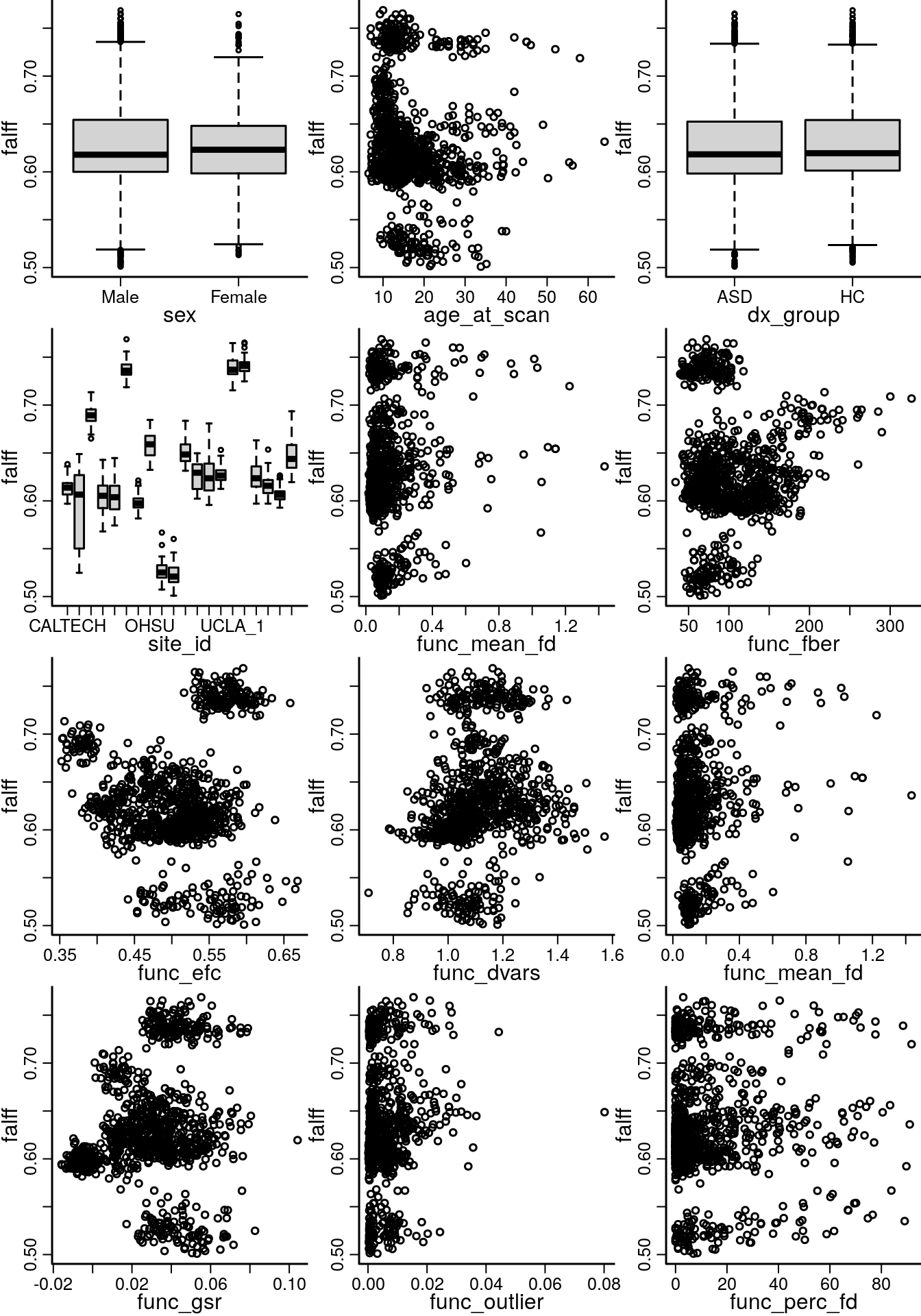
Figure 4.1: Marginal plots for mean of the outcome image and each variable considered for the image level model.
model = lm(as.formula(paste('meanY ~', paste(potentialVars, collapse='+'))), data=dat)library(car) # for avPlots
par(mar=c(3,3,0,0))
avPlots(model, terms=~.-site_id, main=paste('Whole brain', derivative), layout=c(4,3), ask=FALSE, mgp=c(1.8, 0.7, 0)) 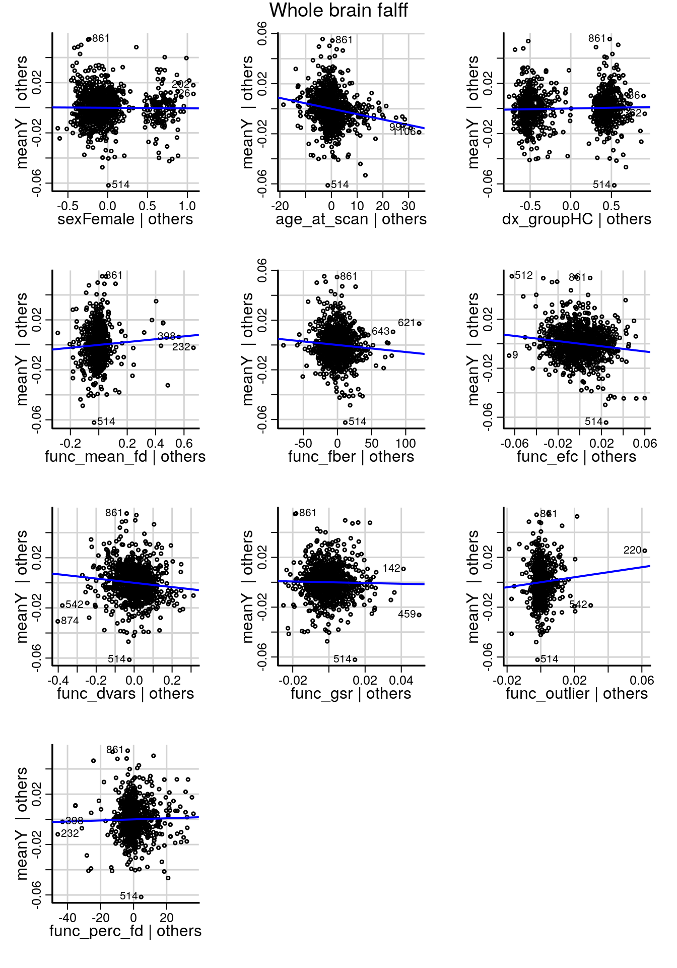
Figure 4.2: Added variable plots for demographic, behavioral and imaging covariates that show the relationship between each variable and the outcome (meanY) cintrolling for the other variables in the model.
4.1.2 Voxel-wise analysis with lmPBJ
The following code sets up variables we will use to analyze the data. We assume that the mean value of fALFF for people in the population is a linear function of sex, diagnostic group, site where the data were collected, and the motion covariates. We will compare this to a model that does not include diagnosis and another model that does not include age, so that we are testing for the effect of diagnosis and age separately at each location in the fALFF image. In addition, we will include weights for each participant that are proportional to the inverse of the the person’s mean frame displacement during the scan with the logic being that participants that move more will have noisier data (S. N. Vandekar et al. 2019). These weights correspond to a working variance structure, i.e. they are an estimate of how we think the variance of the imaging data differs across study participants. If we use robust standard error estimates, then the weights do not have to be correctly specified as the inverse of the variance for each participant; more details are given below and in PBJ analysis methods.
The mask file that was created above will be used to specify where in the image the analysis should be performed. The output file indicates where to save the output of pbjInference later in the analysis, and ncores controls how many cores will be used to perform the analysis.
Finally, we include two example vectors of cluster forming thresholds that will be used for inference later.
# need age_at_scan in both models for testing nonlinear functions
form = paste0(" ~ sex + age_at_scan + func_mean_fd + func_fber + func_outlier + dx_group + site_id" )
formred = paste0(" ~ sex + age_at_scan + func_mean_fd + func_fber + func_outlier + site_id")
formredAge = paste0(" ~ sex + dx_group + func_mean_fd + func_fber + func_outlier + site_id")
#  weights for each subject. Can be a character vector
weights = "func_mean_fd"
mask = maskfile
output = paste0(tempfile(), '.rdata')
ncores = 24
The following line fits the model and estimates the coefficient and test statistic for the diagnosis variable. By default, lmPBJ uses robust standard errors, which provide consistent standard error and RESI estimates, even if the weights, covariance structure, and mean model are not correctly specified. This means that the results are not sensitive to differences in variance structure related to diagnosis, motion, or site.
This option can be changed by setting the robust argument to FALSE.
The transform argument defaults to t; this means the test statistics are assumed to be approximately T-distributed at each voxel, and it converts to chi-squared statistics by converting them to \(Z\) statistics and squaring them.
The template file is not required, but makes visualization easier down-the-road.
We can perform a similar analysis of age, using the same full model as input, but using the reduced formula with age removed.
# DX analysis
abideDX = lmPBJ(dat$files, form=form, formred=formred, mask=mask, data=dat, Winv=dat[,weights], template = templatefile)
abideDX
## Full formula: ~ sex + age_at_scan + func_mean_fd + func_fber + func_outlier + dx_group + site_id
## Reduced formula: ~ sex + age_at_scan + func_mean_fd + func_fber + func_outlier + site_id
## 30272 voxels in mask
## StatMap quantiles (0, 0.01, 0.05, 0.95, 0.99, 1):
## [ 0, 0, 0.01, 5.32, 9.18, 21.05 ]
## sqrtSigma:
## [n = 1025 ; df = 1 ; rdf = 999 ]
## id variable is:
## NULL
## lmPBJ inference settings:
## robust = TRUE ; HC3 = TRUE ; transform = t
## pbjInference not run yet.# Age analysis
abideAge = lmPBJ(dat$files, form=form, formred=formredAge, mask=mask, data=dat, Winv=dat[,weights], template = templatefile)Printing the fitted statMap object at the terminal gives information about how the model was fit and the output values.
We can visualize the results using a lightbox view with the image function, which calls the image.statMap method for objects of class statMap (Figure 4.3).
The argument cft_p=0.05 indicates to show only regions with an uncorrected \(p\)-value less than \(0.05\).
image(abideDX, cft_p=0.05, crop=TRUE)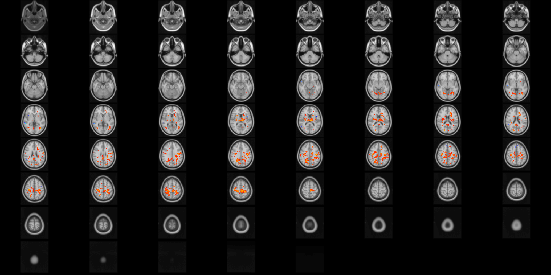
Figure 4.3: Diagnostic differences in fALFF controlling for sex, age, motion, and site. Colors are signed -log10(p) values showing uncorrected \(p \le 0.05\).
If the parameter tested is 1-dimensional (such as a T-test), the results are shown by default as signed \(-log_{10}(p)\). The results show clusters in posterior cingulate and parietal lobes that are positively associated with ASD diagnosis, as well as small clusters at the midline that are possibly due to motion artifact. The second call to image passes additional named arguments to the image.niftiImage function to more easily visualize the results (Figure 4.4).
image(abideDX, cft_p=0.05, plane='coronal', index=seq(28, length.out=8), nrow=2, crop=FALSE)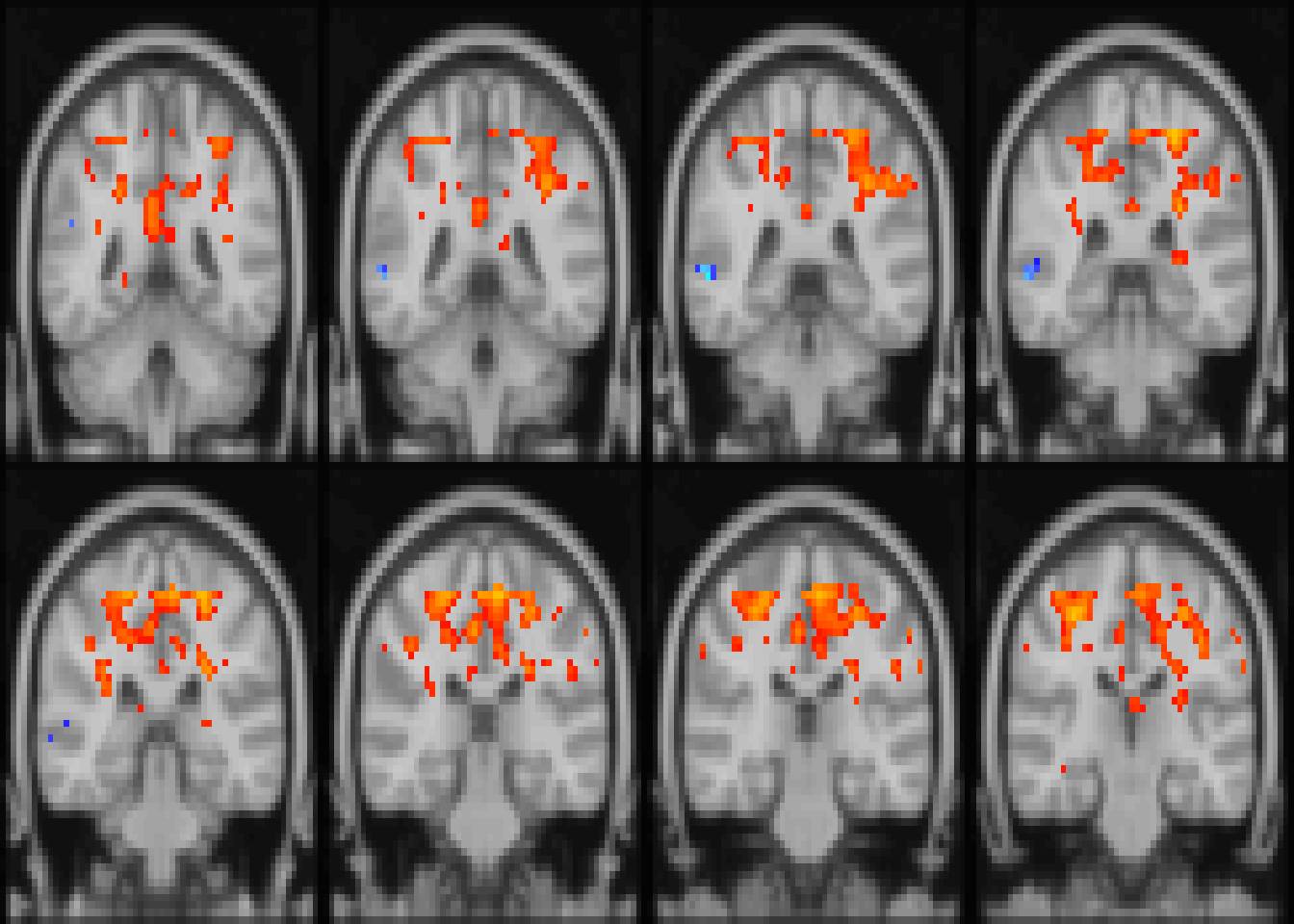
Figure 4.4: Diagnostic differences in fALFF controlling for sex, age, motion, and site. Colors are signed -log10(p) values showing uncorrected \(p \le 0.05\). for slices z=28:36
We can also visualize the same result on the effect size scale using the same function with the cft_s=0.1 argument, which highlights regions where the effect size, \(S\), is larger than \(0.1\) (a small effect size; Figure 4.5; see Section REF).
image(abideDX, cft_s=0.1, plane='sagittal', index=seq(28, length.out=8), nrow=2)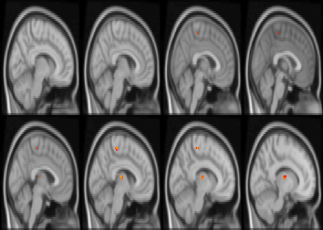
Figure 4.5: Diagnostic differences in fALFF controlling for sex, age, motion, and site. Colors are signed RESI values showing uncorrected \(S \ge 0.1\). for slices z=28:36.
The age analysis highlights regions of the brain in prefrontal cortex where there are differences associated with age, with estimated effect sizes larger than \(S=0.1\) and \(S=0.15\) (Figures 4.6 and 4.7). Blue is negative and highlights regions where the reduction in fALFF has an effect size larger than \(S=0.1\).
image(abideAge, cft_s = 0.1, index=20:49)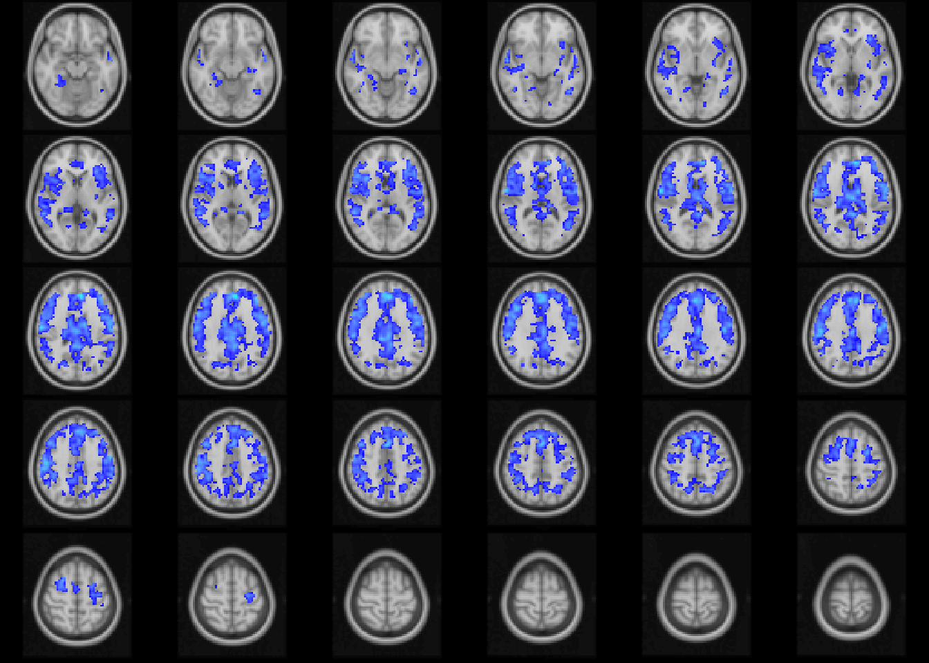
Figure 4.6: Age-related differences in fALFF controlling for sex, diagnosis, motion, and site. Colors are signed RESI values showing uncorrected \(S\ge 0.1\). for slices z=20:49.
image(abideAge, cft_s = 0.15, index=14:49, plane='sagittal')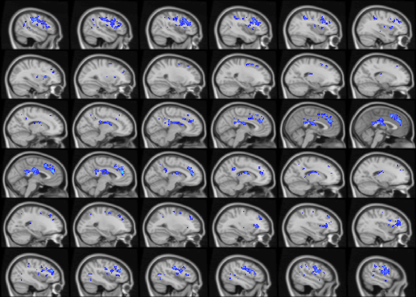
Figure 4.7: Age-related differences in fALFF controlling for sex, diagnosis, motion, and site. Colors are signed RESI values showing uncorrected \(S \ge 0.1\). for slices x=14:49.
4.1.3 Topological inference (Maxima, CEI, CMI)
Here, we will perform inference on local maxima, cluster extent inference (CEI), and cluster mass inference (CMI) on the statistical images for the diagnosis and age effects.
These forms of statistical inference take a cluster forming threshold (CFT) as input and compute the probability that a cluster of the given size (or mass) would appear if there is no association
Cluster size is the number of voxels in a given spatially contiguous cluster above the CFT and cluster mass is the sum of the statistical values in the spatially contiguous above the CFT.
Inference procedures are run in the pbj package using the pbjInference command.
This function runs the inference in the foreground or background, serially or in parallel, and returns an statMap object that is the original statMap object, with the a pbj object added as a new element of the list.
The following command runs CEI and CMI on the diagnosis statistical image in the background in parallel using 24.
The pbjInference takes the statMap object from lmPBJ as input.
It automatically runs in the background if the user passes an .rdata or .rds file.
The if statement checks if the file exists to avoid running it twice.
The mc.cores argument specifies how many cores to run in parallel.
As described in @ref{#pbjInference}, the statistic argument is the most important and determines what type of inference to run on the images.
The default is statistic=mmeStat, which can be used for inference of local maxima and clusters.
pbjInference takes named arguments that getp passed to the statistic function. In this case CEI=TRUE, CMI=TRUE, maxima=TRUE instruct pbjInference to run all types of inference procedures on the diagnosis image.
Other arguments can be found by typing ?mmeStat at the command line.
Finally, the cft_s=0.1 argument specifies that we are targeting inference on clusters where the effect size is larger that \(S=0.1\), which corresponds to a Cohen’s \(d=0.2\) (S. Vandekar, Tao, and Blume 2020).
rdatafile = file.path(datadir, 'abide/results/abideDX.rdata')
# make sure the directory exists
dir.create(dirname(rdatafile), showWarnings = FALSE)
if(!exists(rdatafile)){
  progr = pbjInference(abideDX, rdata_rds = rdatafile, mc.cores=ncores, CEI=TRUE, CMI=TRUE, maxima=TRUE, cft_s=0.1)
}
The code below runs the same inference procedure to investigate the age effect using two effect size thresholds to target effect sizes larger than \(S=0.1\) and \(S=0.15\). These thresholds should be determined in advance. See Selecting effect size CFTs.
In addition we change is the output filename and the input statMap object to abideAge.
rdatafile = file.path(datadir, 'abide/results/abideAge.rdata')
if(!exists(rdatafile)){
  progr = pbjInference(abideAge, rdata_rds = rdatafile, mc.cores=ncores, CEI=TRUE, CMI=TRUE, maxima=TRUE, cft_s=c(0.1, 0.15) )
}
4.1.4 Interpreting and visualizing pbjInference results
4.1.4.1 Tabulating inference results
After fitting the model we can use the table.statMap function to visualize the results using a cluster or maxima summary table.
The cluster summary table gives the cluster index, which is based on the physical coordinate of the cluster in the image, the cluster or maxima statistical value, the voxel coordinates of the centroid, the unadjusted \(p\)-value, FWER adjusted \(p\)-value, and the effect size (RESI; Tables 4.8, 4.9, and 4.10).
For the maxima table, only the global maxima is computed in each bootstrap by default due to the computational demand of computing local maxima, so only the FWER adjusted results are available (Table 4.10).
Details on the estimation and interpretation of the \(p\)-values are given in Statistical Inference.
The table results are visualized using the reactable package, but can easily be exported to .csv files for journal formatting.
In this case, because ABIDE has a large sample size of 1025, the cluster-based inference \(p\)-values are small even for relatively small cluster sizes (Table 4.8) because an effect size of \(S=0.15\) corresponds to a small cluster forming threshold on the \(p\)-value scale.
rdatafile = file.path(datadir, 'abide/results/abideDX.rdata')
if(file.exists(rdatafile)){
  # loading the rdata file loads "statMap" and "computeTime" objects
  load(rdatafile)
  abideDX = statMap
  ctDX = computeTime[3]
  rm(statMap)

  # create the tables for each inference type
  CEItab = table.statMap(abideDX, cft_s=0.1)
  CMItab = table.statMap(abideDX, method='CMI', cft_s=0.1)
  maximaTab = table.statMap(abideDX, method='maxima')
  #plot(seq(0, 35, length.out=1000), abideDX$pbj$fwerCDF$maxima(seq(0, 35, length.out=1000)), type='l')
} library(reactable)
reactable(CEItab, columns = list(
"Centroid (vox)"=colDef(align = 'right'),
"Unadjusted p-value"=colDef(format = colFormat(digits=3)),
"FWER p-value"=colDef(format = colFormat(digits=3)),
"Max RESI"=colDef(format = colFormat(digits=3))
))Figure 4.8: CEI inference results for the test of the effect of diagnosis on fALFF in the ABIDE data.
  reactable(CMItab, columns = list(
    "Centroid (vox)"=colDef(align = 'right'),
    "Unadjusted p-value"=colDef(format = colFormat(digits=3)),
    "FWER p-value"=colDef(format = colFormat(digits=3)),
    "Max RESI"=colDef(format = colFormat(digits=3))
                                ))
Figure 4.9: CMI inference results for the test of the effect of diagnosis on fALFF in the ABIDE data.
  reactable(maximaTab, columns = list(
    "Coord (vox)"=colDef(align = 'right'),
    "Chi-square"=colDef(format=colFormat(digits=2) ),
    "FWER p-value"=colDef(format = colFormat(digits=3)),
    "Max RESI"=colDef(format = colFormat(digits=3))
                                ))
Figure 4.10: Inference results for local maxima for the test of the effect of diagnosis on fALFF in the ABIDE data.
The same summary tables for age are given below and demonstrate the use of other cluster forming thresholds (RESI; Tables 4.11, 4.12, and 4.13).
rdatafile = file.path(datadir, 'abide/results/abideAge.rdata')
if(file.exists(rdatafile)){
  # loading the rdata file loads "statMap" and "computeTime" objects
  load(rdatafile)
  abideAge = statMap
  ctAge = computeTime[3]
  rm(statMap)

  # create the tables for each inference type
  CEItab = table.statMap(abideAge, cft_s=0.1)
  CEItab15 = table.statMap(abideAge, cft_s=0.15)
  CMItab = table.statMap(abideAge, method='CMI', cft_s=0.15)
  maximaTab = table.statMap(abideAge, method='maxima')
} reactable(CEItab, columns = list(
"Centroid (vox)"=colDef(align = 'right'),
"Unadjusted p-value"=colDef(format = colFormat(digits=3)),
"FWER p-value"=colDef(format = colFormat(digits=3)),
"Max RESI"=colDef(format = colFormat(digits=3))
))Figure 4.11: CEI inference results for the test of the effect of age on fALFF in the ABIDE data.
  reactable(CMItab, columns = list(
    "Cluster Mass"=colDef(format = colFormat(digits=0)),
    "Centroid (vox)"=colDef(align = 'right'),
    "Unadjusted p-value"=colDef(format = colFormat(digits=3)),
    "FWER p-value"=colDef(format = colFormat(digits=3)),
    "Max RESI"=colDef(format = colFormat(digits=3))
                                ))
Figure 4.12: CMI inference results for the test of the effect of age on fALFF in the ABIDE data.
  reactable(maximaTab, columns = list(
    "Coord (vox)"=colDef(align = 'right'),
    "Chi-square"=colDef(format=colFormat(digits=2) ),
    "FWER p-value"=colDef(format = colFormat(digits=3)),
    "Max RESI"=colDef(format = colFormat(digits=3))
                                ))
Figure 4.13: Inference results for local maxima for the test of the effect of age on fALFF in the ABIDE data.
4.1.4.2 Visualizing results
The image function has a special behavior for statMap objects that have had pbjInference run and include a pbj object.
There are numerous options for quickly visualizing the results within R.
Running the image command on the statMap object that has a pbj object automatically visualizes all clusters in the image (Figure 4.14).
By default the image function draws in the axial plane using the CEI results.
The image function defaults to showing the plane at the centroid of the selected cluster and prints the cluster ID number on the center of the cluster.
The slices are ordered by the rows of Table 4.8.
image(abideDX, cft_s=0.1, plane='axial')
# od = tempdir()
# files = write.statMap(abideDX, outdir=od)
# papaya(c(templatefile, files$`CMI 1`))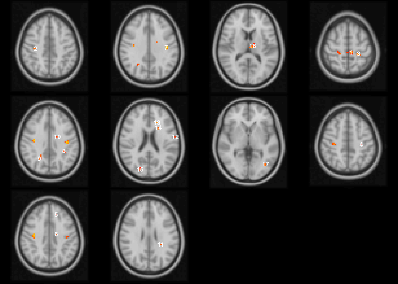
Figure 4.14: Visualization of pbjInference results.
We can see in the first two rows of Table 4.8, that there are two clusters with relatively small FWER adjusted \(p\)-values. We can visualize these using the image function and setting \(\alpha=0.06\) to capture the first two rows (Figure 4.15).
image(abideDX, cft_s=0.1, alpha=0.06)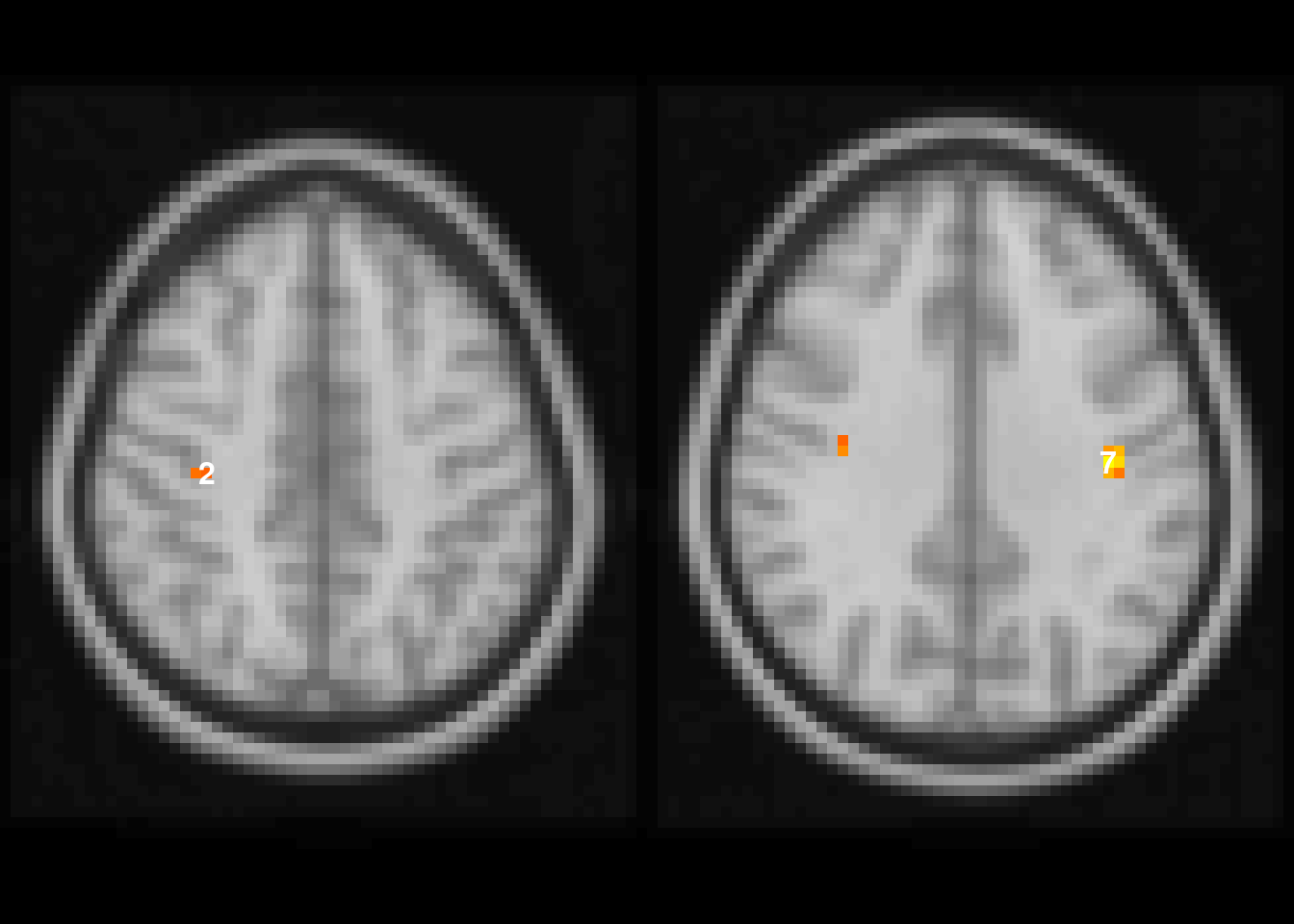
Figure 4.15: Visualization of clusters with FWER adjusted $p<0.06$
# od = tempdir()
# files = write.statMap(abideDX, outdir=od)
# papaya(c(templatefile, files$`CMI 1`))
We can also visualize the first four largest clusters by specifying the ROI index from Table 4.8 (Figure ??). Here, we change the plane and suppress the cluster number overlay.
image(abideDX, cft_s=0.1, roi=c(2,7,16,1), plane='coronal', clusterID=FALSE)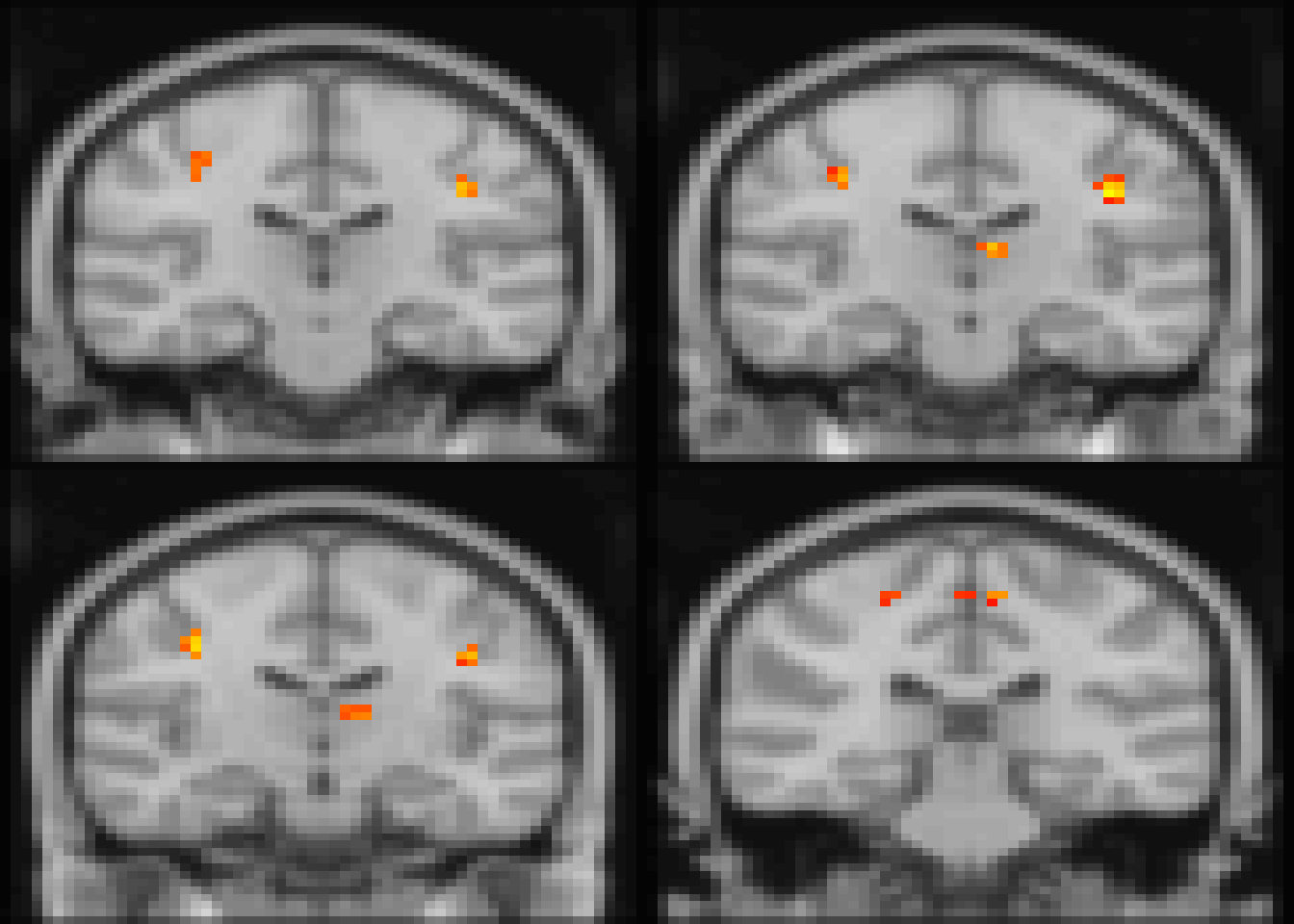
# od = tempdir()
# files = write.statMap(abideDX, outdir=od)
# papaya(c(templatefile, files$`CMI 1`))
4.1.4.3 Plotting results
library(ggplot2)
layout(matrix(1:2, nrow=1))
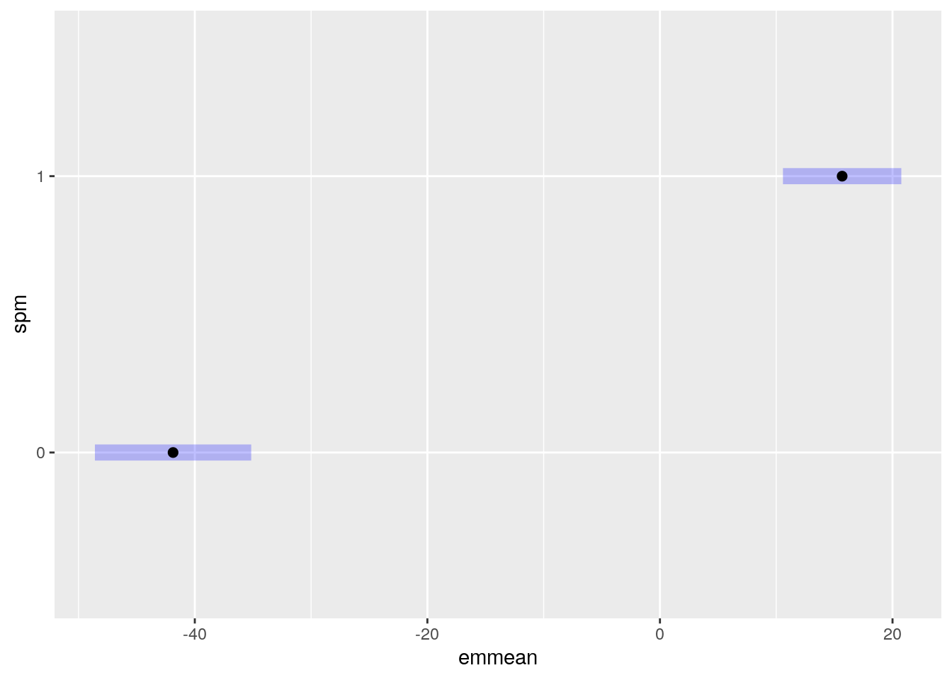
abideDXem = plotData.statMap(abideDX, emForm = ~ dx_group)
plot(abideDXem$emmeans[[1]], horizontal=FALSE, ylab='Diagnosis' ) +
  ggtitle(paste('ROI', names(abideDXem$emmeans)[[1]]))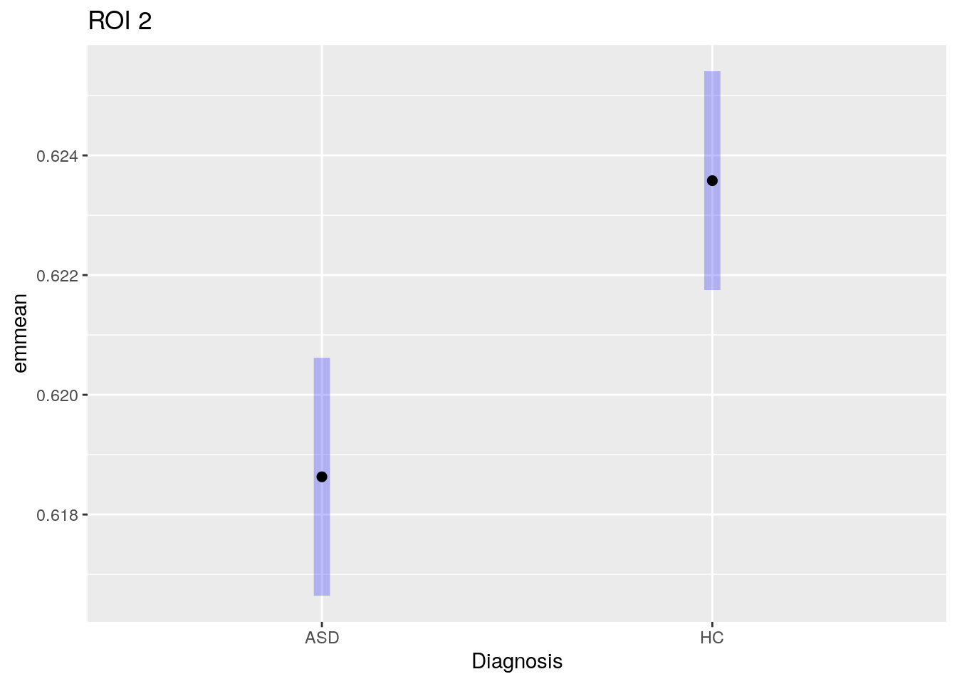
# + geom_jitter(data=abideDXem$data, aes(x = roi2, y=ifelse(dx_group=='ASD', 1, 2)), size=0.5, width=0.1)
plot(as.factor(abideDXem$data$dx_group), abideDXem$data$roi2, xlab='Diagnosis', ylab='fALFF')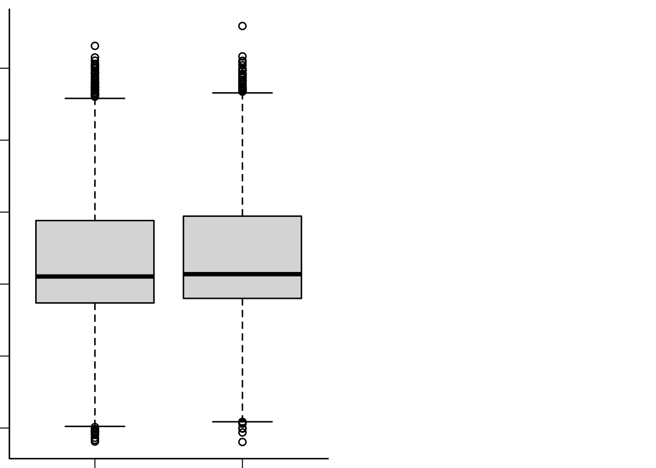
ageRange = range(abideAge$data$age_at_scan)
abideAgeEM = plotData.statMap(abideAge, method='CEI', cft_s=0.15, emForm = ~ age_at_scan, at=list(age_at_scan = seq(ageRange[1], ageRange[2], length.out=100)) )

# create the plot of ROI10 using base R
plot(abideAgeEM$data$age_at_scan, abideAgeEM$data$roi10, xlab='Age', ylab='fALFF', pch=20, main='Age effect in Cluster 10')
plotDF = as.data.frame(abideAgeEM$emmeans[[1]])
polygon(c(plotDF[,'age_at_scan'], rev( plotDF[,'age_at_scan'])), c(plotDF[,'lower.CL'], rev(plotDF[,'upper.CL'])), border=NA, col='gray')
lines(plotDF[,'age_at_scan'], plotDF[,'emmean'])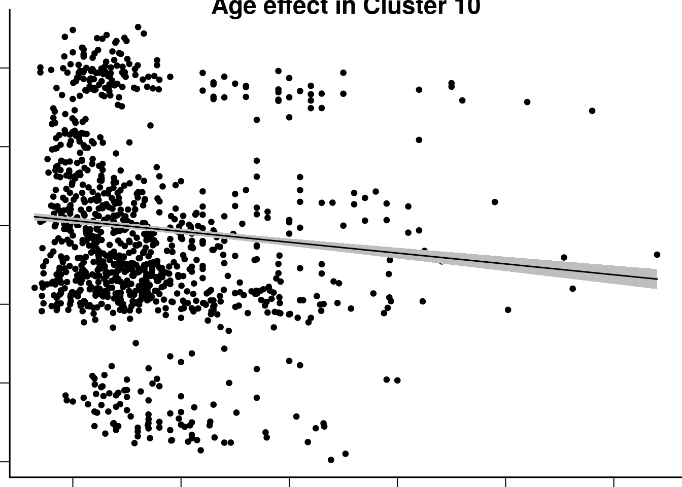
4.1.4.4 Exporting results
The output can be written using the write.statMap function, which writes the statistical image (as \(-\log_{10}(p)\), the RESI \(S\), or the Chi-squared statistical values), the 4D coefficient image, the model information stored in a sqrtSigma object, and then all of the inference results returned by pbjInference. write.statMap returns a list of file paths for all the objects written.
The results are then easily visualized in another software package, if preferred by the user.
statmapFolder = tempfile() # generate a random file folder name
dir.create(statmapFolder) # create the directory
files = write.statMap(abideAge, outdir=statmapFolder) # write the statistical image
## Writing stat and coef images.## Warning in asNifti.default(image, template, internal = TRUE): Ignoring invalid
## internal pointer## Warning in asNifti.default(image, template, datatype, internal = FALSE):
## Ignoring invalid internal pointer## Writing sqrtSigma object.## Writing inference images.## Warning in asNifti.default(image, template, internal = TRUE): Ignoring invalid
## internal pointer## Warning in asNifti.default(image, template, internal = TRUE): Ignoring invalid
## internal pointer
## Warning in asNifti.default(image, template, internal = TRUE): Ignoring invalid
## internal pointer
## Warning in asNifti.default(image, template, internal = TRUE): Ignoring invalid
## internal pointer
## Warning in asNifti.default(image, template, internal = TRUE): Ignoring invalid
## internal pointer
## Warning in asNifti.default(image, template, internal = TRUE): Ignoring invalid
## internal pointer
## Warning in asNifti.default(image, template, internal = TRUE): Ignoring invalid
## internal pointer
## Warning in asNifti.default(image, template, internal = TRUE): Ignoring invalid
## internal pointer
## Warning in asNifti.default(image, template, internal = TRUE): Ignoring invalid
## internal pointer
## Warning in asNifti.default(image, template, internal = TRUE): Ignoring invalid
## internal pointer4.1.4.5 Interative visualization
The Papaya widget in Neuroconductor allows us to embed the papaya image viewer in an html document for interactive visualization.
The papaya image viewer takes a vector of image paths as input for the background and overlay images.
Here, we use the output from write.statMap to visualize the results on the signed \(-\log_{10}(p)\) scale.
library(papayaWidget)
papaya(c(templatefile, files$stat )) # view the statistical image
4.2 Pain meta-analysis
The pain21 R package is a dataset of coefficient and variance maps from 21 pain studies obtained from the “21 Pain Studies” Neurovault repository [maumet_sharing_2016].
For this analyses, we will perform a meta-analysis to estimate regions that are activated above a given effect size threshold.
Often, public data sets only include standardized statistical maps; this makes meta-analysis using conventional methods (e.g. mixed effects models) difficult or impossible because the study level variances aren’t known. However, the sPBJ procedure is still valid in large samples because it uses robust standard errors, so any weights can be used and the standard errors are still consistent, as long there is an adequate number of studies used in the analysis. The best weight vector for the model is one that is a good estimate of the variance for the statistical map for that study, we do that below. However, we can also see how inference changes if we don’t have the variance images, but assume instead that the variance of the estimate from each study is proportional to the sample size.
library(pain21)
pain = pain21()
pain$mask
## [1] "/home/vandeks/R/x86_64-pc-linux-gnu-library/4.0/pain21/pain21/mask.nii.gz"The pain21 function from the pain21 package creates a data frame with file paths for the imaging data that we need to perform the analysis. The following images are required to perform the analysis:
- The mask image is a binary image indicating which voxels should be included in the analysis.
- The character vector of images is the contrast image from each study included in the meta-analysis.
- The character vector of varimages contains the voxel level estimates of variance from each study.
The template is the MNI 152 template and is not necessary to compute the statistical map or perform SEI, but it is handy to include here for visualization in later steps. The code below loads the data and shows the names of the images.
library(pain21)
pain = pain21()
basename(pain$mask)
## [1] "mask.nii.gz"basename(pain$template)## [1] "MNI152_T1_2mm_brain.nii.gz"head(basename(pain$data$images))## [1] "contrast_pain_01.nii.gz" "contrast_pain_02.nii.gz"
## [3] "contrast_pain_03.nii.gz" "contrast_pain_04.nii.gz"
## [5] "contrast_pain_05.nii.gz" "contrast_pain_06.nii.gz"head(basename(pain$data$varimages))## [1] "var_pain_01.nii.gz" "var_pain_02.nii.gz" "var_pain_03.nii.gz"
## [4] "var_pain_04.nii.gz" "var_pain_05.nii.gz" "var_pain_06.nii.gz"Below, we compute the mean variance of the coefficient image for each study and use the inverse variance as a weights in the meta-analysis model.
This assumes that the variance of the coefficient image estimator at each voxel is proportional to the inverse of the mean of the variance.
While this assumption is likely incorrect, it might be a good working model. Using the robust=TRUE option ensures that the standard error estimators for the meta-analysis model are consistent, despite this potentially incorrect assumption.
If the weights are a good working model, it will improve efficiency (i.e. reduce the variance of the coefficient, effect size, and standard error estimators) relative to using an unweighted model.
The square root of the variance of the coefficient estimate is mathematically linearly related to the square root of the sample size (Figure 4.16). This may vary across samples due to sampling variability, or differences in the efficiency of the design of the study. In the absence of having the inverse variance image, we could use inverse sample sizes as weights for the meta-analysis.
The last few lines use lmPBJ to fit a series of different meta-analysis models.
The first estimates the mean activation of the brain across similarly conducted pain studies.
By default, the model is fit with the robust=TRUE option, which means that the consistent standard error estimator are used for the coefficient.
The full model is an intercept only model (estimating the mean activation across studies) and compares this to a null model with no mean. This tests whether the activation at a given location is different than zero.
The painSPM lmPBJ call compares the estimates across the SPM and FSL software versions to contrast differences in the pain activation maps between software versions.
The painN call tests the association of sample size (n) with the estimated brain response for each study. This test is to probe publication bias; if there is publication bias, we might expect smaller studies to report larger effect sizes on average because larger effect size estimates are required to obtain small p-values in smaller samples.
library(pbj)
outdir = dirname(tempdir())


library(RNifti) # NIfTI IO
# read in variance images and compute whole brain average variance to use as weights
varimages = readNifti(pain$data$varimages)
pain$data$Winv = sapply(1:length(varimages), function(ind){
  mean(varimages[[ind]][varimages[[ind]]!=0])
})
images = readNifti(pain$data$images)
pain$data$mean = sapply(1:length(images), function(ind){
  mean(images[[ind]][images[[ind]]!=0])
})

plot(sqrt(pain$data$n), sqrt(pain$data$Winv), xlab='Sample size', ylab='Inverse variance', main = 'Variance-sample size', bty='l')
abline(lm(sqrt(Winv) ~ sqrt(n), data=pain$data))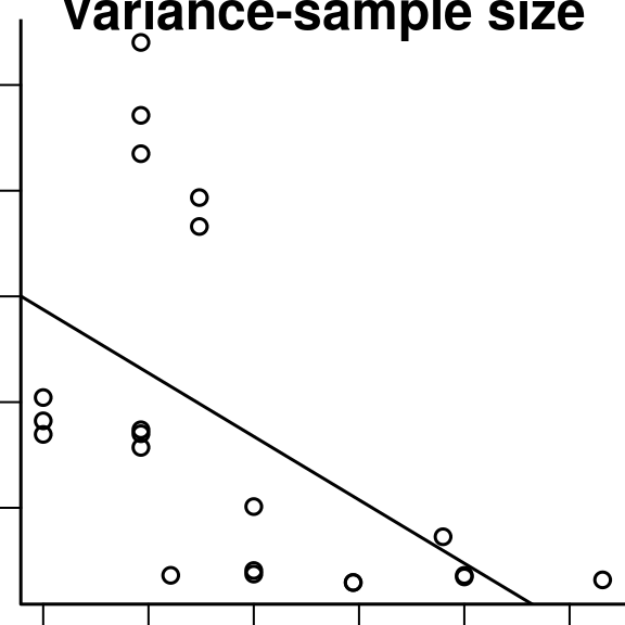
Figure 4.16: Relationship between mean of the square root of the average of the variance image and the sample size across the 21 pain studies.
# plot(pain$data$spm, pain$data$Winv)
# plot(pain$data$spm, pain$data$mean)

# fit an intercept only model and test the intercept
painPBJ <- lmPBJ(pain$data$images, form = ~1, formred = NULL, pain$mask,
                 data = pain$data, Winv = pain$data$Winv, template = pain$template)

# fit a model comparing results between software version
painSPM <- lmPBJ(pain$data$images, form = ~1 + spm, formred = ~ 1, pain$mask,
                 data = pain$data, Winv = pain$data$Winv, template = pain$template)

# fit a model for the association between sample size and effect size
painN <- lmPBJ(pain$data$images, form = ~1 + spm + n, formred = ~ 1  + spm, pain$mask,
data = pain$data, Winv = pain$data$Winv, template = pain$template)4.3 NKI-RS analysis
In this tutorial, we use the pbj package to model sex differences age-related changes in gray matter in the cross-sectional Nathan Kline Institute Rockland Sample (NKI-RS). The dataset includes 683 participants ages 6-85.
The outcome images are voxel-based morphometry (VBM).
The intensity of each voxel is a point-wise estimate of gray matter volume [ashburner_computational_2009].
4.3.1 Loading data and basic image processing
The data file can be loaded into R from a .csv file.
# sets path for data file
dbdatafile = '/media/disk2/pbj/data/rockland/demographic/RocklandBehavioral.csv'
# load in data file
nki = read.csv(dbdatafile, stringsAsFactors = TRUE)
We do some minor data curation by subsetting the dataset to subjects who have data on the server (data that did not pass quality assurance was not installed at this location) and listing the first Nifti image file for each subject. We add two other columns to the dataset for creating downsampled images (from 1mm to 2mm isotropic resolution) and creating 8mm FWHM Gaussian smoothed images. Lastly, we add columns for age and sex from the variables included in the NKI-RS.
The commented code shows how the mask file was made, as the intersection of all voxels that are above zero in all of the participants’ images.
maskfile = "/media/disk2/pbj/data/rockland/neuroimaging/overlap_mask_2mm.nii.gz"
templatefile = '/usr/local/fsl/data/standard/MNI152_T1_2mm_brain.nii.gz'
# reads in image and creates lightbox view.
image(readNifti(templatefile))
library(papayaWidget)

## CREATE MASK
# if(!file.exists(maskfile)){
#   imgs = readNifti(nki$files)
#   mask = imgs[[1]]
#   mask[,,] = 0
#   imgs = apply(simplify2array(imgs), 1:3, function(v) sum(v>0))
#   mask[sum(imgs)==nrow(nki)] = 1
#   writeNifti(mask, file=maskfile)
# }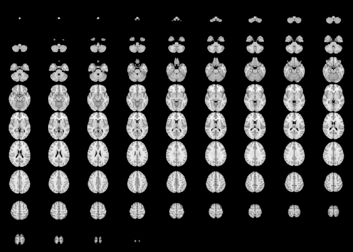
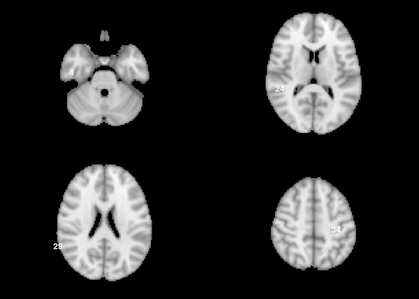
Figure 4.21: Lightbox view of the template image. This is the default display for niftiImage objects.
PUT THIS SOMEWHERE ELSE BELOW.
# location to save results
pbjdatafile = '/media/disk2/pbj/pbj_ftest/nkirs_bootstrap_results.rdata'
permdatafile = '/media/disk2/pbj/pbj_ftest/nkirs_permutation_results.rdata'
The input VBM data are at 1mm isotropic resolution and unsmoothed.
The code below downsamples the images to 2mm isotropic resolution and applies smoothing at 8mm FWHM. It first checks whether the downsampled, smoothed output files exist; if not, it downsamples and applies smoothing using functions from the fslr package.
The second to last line creates an interactive viewer embedded into this html document using papayaWidget to visualize the effect of the smoothing in the first participant.
if(!all(file.exists(nki$files2mmsm8))){
  ## CREATE DOWNSAMPLED DATA
  invisible(mcmapply(flirt, infile=nki$files, outfile=nki$files2mm, opts = '-applyxfm', MoreArgs=list(reffile=templatefile, retimg=FALSE), mc.cores = ncores ))
  ## SMOOTH DOWNSAMPLED DATA
  # convert FWHM to sigma
  sigma = 8/2.355
  invisible(mcmapply(susan, file=nki$files2mm, outfile=nki$files2mmsm4, MoreArgs=list(sigma=sigma, dimg='3', n_usans='0'), mc.cores=ncores))
  # sigma = 8: using 8mm smoothing
}

# view files
# set downsampled smoothed files as the main file
papaya(c(templatefile, nki$files2mm[1], nki$files2mmsm8[1]))
4.3.2 Model specification
In order to study sex differences in the mean adult life-span curve of gray matter volume we fit the model \[ Y_i(v) = \alpha_0(v) + \alpha_1(v)\text{sex}_i + f_1(\text{age}_i, v) + \text{sex}_i \times f_2(\text{age}_i, v) + E_i(v), \] where \(Y_i(v)\) denotes the VBM image for participant \(i\) and voxel location \(v\). \(\text{sex}_i\) is an indicator variable that is equal to 1 if participant \(i\) is a male. We fit \(f_1\) and \(f_2\) with natural cubic splines on 4 degrees of freedom. The unknown parameters \(\alpha_0(v)\), \(\alpha_1(v)\), \(f_1\), and \(f_2\) quantify the association between each variable and the VBM image at location \(v\).
To study sex differences in the life-span curve, we test the nonlinear age by sex interaction which corresponds to parameters that control the shape of the function \(f_2\). The null hypothesis is that \(f_2(\text{age}_i) = 0\) for all values of \(\text{age}_i\) and all voxel locations \(v\), versus the alternative hypothesis that this is not true, \[\begin{align*} H_0: & f_2(\text{age}, v) = 0 \\ H_1: & f_2(\text{age}, v) \ne 0. \end{align*}\] Because \(f_2\), is modeled with 4 degrees of freedom the test for \(H_0\) is an F-test at each voxel location, \(v\), on 4 degrees of freedom.
This model specification is used to test the nonlinear age by sex interaction. The null hypothesis at each location is that males and females follow the same developmental trajectory. The third line subsets the data to rows that have no missing variables (complete case analysis).
nki$files = nki$files2mmsm8
# Testing the interaction between nonlinear age x sex
lmfull =  ~ ns(age, df=4) * sex
lmred = ~ sex + ns(age, df = 4)
nki = nki[apply(!is.na(nki[,all.vars(as.formula(lmfull))]), 1, all), ]

# add a demographic summary table using tangram
table1( ~ age | sex, data=nki)| Female (N=422) |
Male (N=260) |
Overall (N=682) |
|
|---|---|---|---|
| age | |||
| Mean (SD) | 45.9 (20.7) | 38.0 (22.2) | 42.9 (21.6) |
| Median [Min, Max] | 49.5 [6.18, 85.6] | 30.2 [6.21, 84.8] | 45.1 [6.18, 85.6] |
To test the parameters corresponding to the \(f_2\), we use a robust test statistic.
The model is fit using the lmPBJ function and computes the coefficients, the robust test statistic, and objects required to perform inference in the next step.
# lmPBJ -- fits the model and computes the statistical image for the covariate of interest
## using robust test statistics (`robust = TRUE`)
robustStatMap <- lmPBJ(nki$files, form=lmfull, formred=lmred, mask=maskfile, template = templatefile, data=nki, robust = TRUE, HC3 = TRUE, transform = 't')
The result from this command is an object of class statMap that contains the following objects:
statis a vector the test statistics values for all voxels in the mask.coefis a matrix of the parameters tested for all voxels in the mask.sqrtSigmais a list of objects that contain everything required to perform statistical inference in the next step. It includes settings that the user chose when running thelmPBJcommand and features of the test statistic, such as the degrees of freedom and residual degrees of freedom.formulasis a list of the formulas used to runlmPBJ.datais the data set covariates used to fit the model.
4.3.3 Visualizing the results
When multiple parameters are being tested the test statistic is computed as a chi-squared statistical image. We can visualize the image to get an idea of what the results look like before computing p-values for topological features, such as cluster extent p-values.
The image command can be used to create static images at this stage to create figures for papers or quickly visualize the results.
Because the test statistic is approximately chi-square distributed, we can compute uncorrected image thresholds for visualizing the results.
If we want to view where the uncorrected p-value \(p<0.01\), then we can use the command qchisq(0.01, df=robustStatMap$sqrtSigma$df, lower.tail=FALSE)= to obtain an uncorrected threshold for the image.
For convenience, this can be done with the image function by setting the argument cft_p=0.01.
Running image without any arguments defaults to a lightbox view.
Alternatively, the user can specify another plane to visualize, or a set of specific slices.
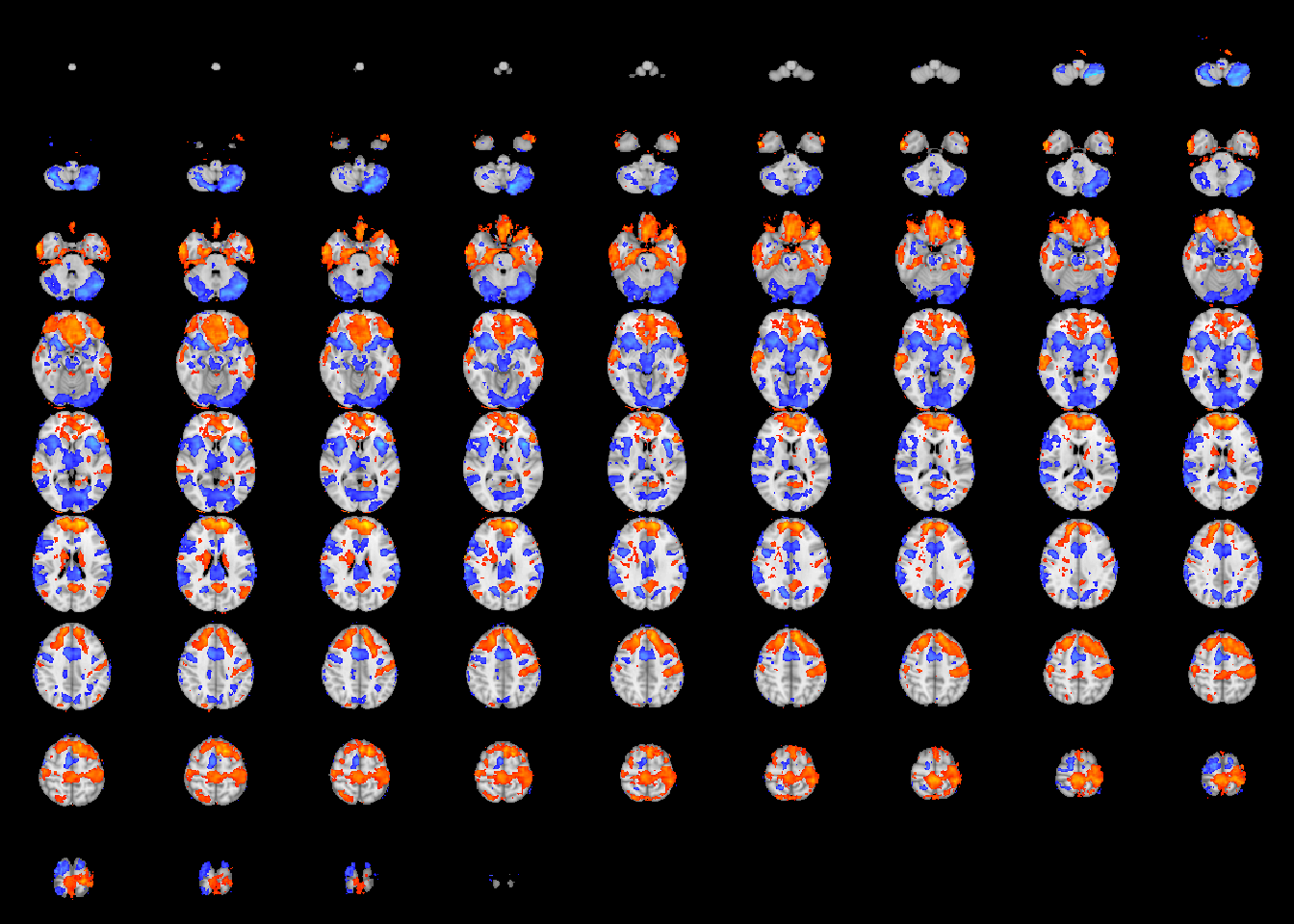
image(robustStatMap, cft_p=0.01)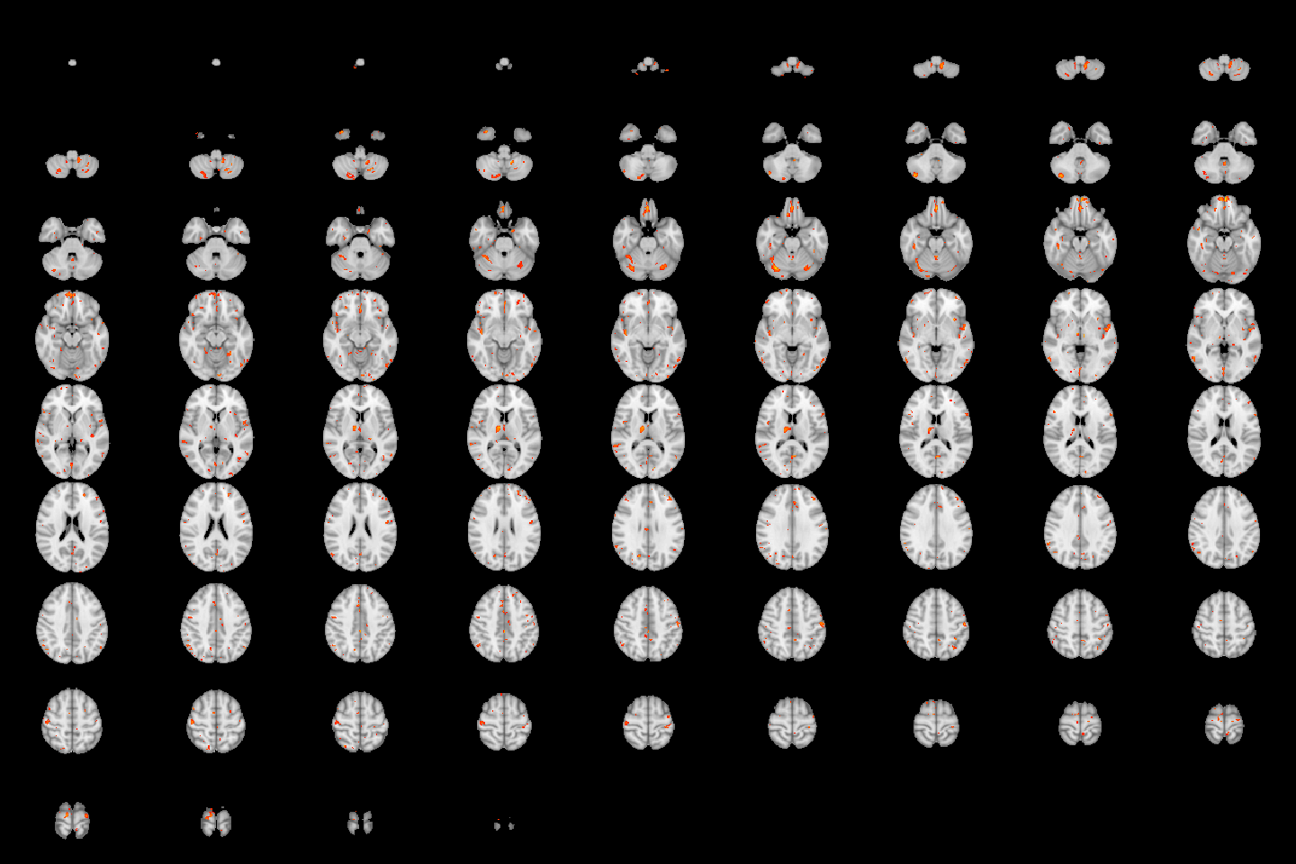
Figure 4.22: Lightbox view of results for the test of the age by sex interaction, with a CFT of \(p=0.01\).
image(robustStatMap, cft_p=0.01, plane = 'sagittal')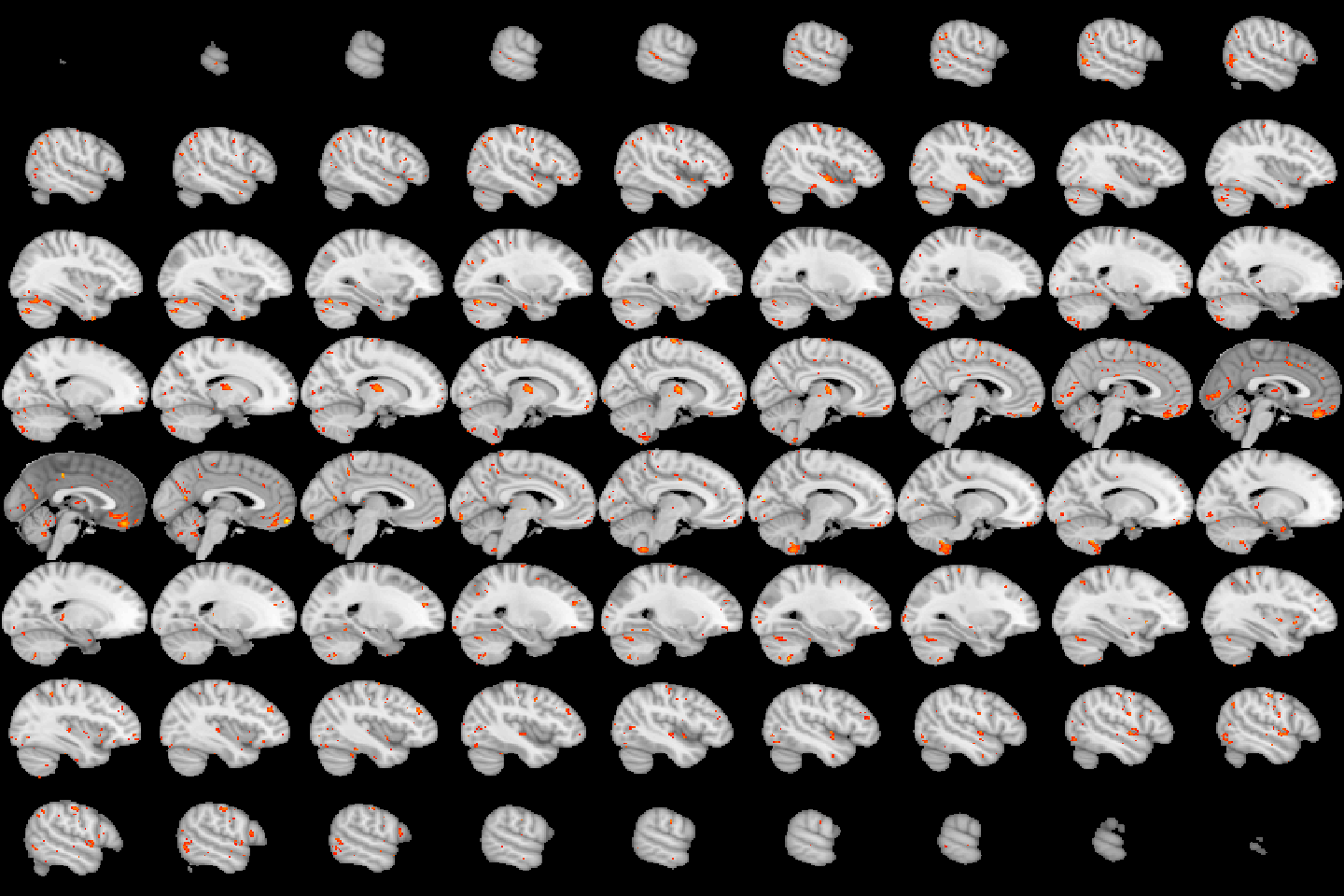
Figure 4.23: Sagittal lightbox view of results for the test of the age by sex interaction, with a CFT of \(p=0.01\).
The base graphics function layout can be used to visualize multiple images in one figure in a custom layout.
# custom layout visualizing inferior frontal cluster
layout(matrix(1:6, byrow=TRUE, nrow=1)); image(robustStatMap, cft_p=0.01, plane = 'axial', slice=25:30)
## Warning in par(...): "slice" is not a graphical parameter## Warning in plot.window(...): "slice" is not a graphical parameter## Warning in plot.xy(xy, type, ...): "slice" is not a graphical parameter## Warning in title(...): "slice" is not a graphical parameter## Warning in plot.window(...): "slice" is not a graphical parameter## Warning in plot.xy(xy, type, ...): "slice" is not a graphical parameter## Warning in title(...): "slice" is not a graphical parameter## Warning in plot.window(...): "slice" is not a graphical parameter## Warning in plot.xy(xy, type, ...): "slice" is not a graphical parameter## Warning in title(...): "slice" is not a graphical parameter## Warning in plot.window(...): "slice" is not a graphical parameter## Warning in plot.xy(xy, type, ...): "slice" is not a graphical parameter## Warning in title(...): "slice" is not a graphical parameter## Warning in plot.window(...): "slice" is not a graphical parameter## Warning in plot.xy(xy, type, ...): "slice" is not a graphical parameter## Warning in title(...): "slice" is not a graphical parameter## Warning in plot.window(...): "slice" is not a graphical parameter## Warning in plot.xy(xy, type, ...): "slice" is not a graphical parameter## Warning in title(...): "slice" is not a graphical parameter## Warning in plot.window(...): "slice" is not a graphical parameter## Warning in plot.xy(xy, type, ...): "slice" is not a graphical parameter## Warning in title(...): "slice" is not a graphical parameter## Warning in plot.window(...): "slice" is not a graphical parameter## Warning in plot.xy(xy, type, ...): "slice" is not a graphical parameter## Warning in title(...): "slice" is not a graphical parameter## Warning in plot.window(...): "slice" is not a graphical parameter## Warning in plot.xy(xy, type, ...): "slice" is not a graphical parameter## Warning in title(...): "slice" is not a graphical parameter## Warning in plot.window(...): "slice" is not a graphical parameter## Warning in plot.xy(xy, type, ...): "slice" is not a graphical parameter## Warning in title(...): "slice" is not a graphical parameter## Warning in plot.window(...): "slice" is not a graphical parameter## Warning in plot.xy(xy, type, ...): "slice" is not a graphical parameter## Warning in title(...): "slice" is not a graphical parameter## Warning in plot.window(...): "slice" is not a graphical parameter## Warning in plot.xy(xy, type, ...): "slice" is not a graphical parameter## Warning in title(...): "slice" is not a graphical parameter## Warning in plot.window(...): "slice" is not a graphical parameter## Warning in plot.xy(xy, type, ...): "slice" is not a graphical parameter## Warning in title(...): "slice" is not a graphical parameter## Warning in plot.window(...): "slice" is not a graphical parameter## Warning in plot.xy(xy, type, ...): "slice" is not a graphical parameter## Warning in title(...): "slice" is not a graphical parameter## Warning in plot.window(...): "slice" is not a graphical parameter## Warning in plot.xy(xy, type, ...): "slice" is not a graphical parameter## Warning in title(...): "slice" is not a graphical parameter## Warning in plot.window(...): "slice" is not a graphical parameter## Warning in plot.xy(xy, type, ...): "slice" is not a graphical parameter## Warning in title(...): "slice" is not a graphical parameter## Warning in plot.window(...): "slice" is not a graphical parameter## Warning in plot.xy(xy, type, ...): "slice" is not a graphical parameter## Warning in title(...): "slice" is not a graphical parameter## Warning in plot.window(...): "slice" is not a graphical parameter## Warning in plot.xy(xy, type, ...): "slice" is not a graphical parameter## Warning in title(...): "slice" is not a graphical parameter## Warning in plot.window(...): "slice" is not a graphical parameter## Warning in plot.xy(xy, type, ...): "slice" is not a graphical parameter## Warning in title(...): "slice" is not a graphical parameter## Warning in plot.window(...): "slice" is not a graphical parameter## Warning in plot.xy(xy, type, ...): "slice" is not a graphical parameter## Warning in title(...): "slice" is not a graphical parameter## Warning in plot.window(...): "slice" is not a graphical parameter## Warning in plot.xy(xy, type, ...): "slice" is not a graphical parameter## Warning in title(...): "slice" is not a graphical parameter## Warning in plot.window(...): "slice" is not a graphical parameter## Warning in plot.xy(xy, type, ...): "slice" is not a graphical parameter## Warning in title(...): "slice" is not a graphical parameter## Warning in plot.window(...): "slice" is not a graphical parameter## Warning in plot.xy(xy, type, ...): "slice" is not a graphical parameter## Warning in title(...): "slice" is not a graphical parameter## Warning in plot.window(...): "slice" is not a graphical parameter## Warning in plot.xy(xy, type, ...): "slice" is not a graphical parameter## Warning in title(...): "slice" is not a graphical parameter## Warning in plot.window(...): "slice" is not a graphical parameter## Warning in plot.xy(xy, type, ...): "slice" is not a graphical parameter## Warning in title(...): "slice" is not a graphical parameter## Warning in plot.window(...): "slice" is not a graphical parameter## Warning in plot.xy(xy, type, ...): "slice" is not a graphical parameter## Warning in title(...): "slice" is not a graphical parameter## Warning in plot.window(...): "slice" is not a graphical parameter## Warning in plot.xy(xy, type, ...): "slice" is not a graphical parameter## Warning in title(...): "slice" is not a graphical parameter## Warning in plot.window(...): "slice" is not a graphical parameter## Warning in plot.xy(xy, type, ...): "slice" is not a graphical parameter## Warning in title(...): "slice" is not a graphical parameter## Warning in plot.window(...): "slice" is not a graphical parameter## Warning in plot.xy(xy, type, ...): "slice" is not a graphical parameter## Warning in title(...): "slice" is not a graphical parameter## Warning in plot.window(...): "slice" is not a graphical parameter## Warning in plot.xy(xy, type, ...): "slice" is not a graphical parameter## Warning in title(...): "slice" is not a graphical parameter## Warning in plot.window(...): "slice" is not a graphical parameter## Warning in plot.xy(xy, type, ...): "slice" is not a graphical parameter## Warning in title(...): "slice" is not a graphical parameter## Warning in plot.window(...): "slice" is not a graphical parameter## Warning in plot.xy(xy, type, ...): "slice" is not a graphical parameter## Warning in title(...): "slice" is not a graphical parameter## Warning in plot.window(...): "slice" is not a graphical parameter## Warning in plot.xy(xy, type, ...): "slice" is not a graphical parameter## Warning in title(...): "slice" is not a graphical parameter## Warning in plot.window(...): "slice" is not a graphical parameter## Warning in plot.xy(xy, type, ...): "slice" is not a graphical parameter## Warning in title(...): "slice" is not a graphical parameter## Warning in plot.window(...): "slice" is not a graphical parameter## Warning in plot.xy(xy, type, ...): "slice" is not a graphical parameter## Warning in title(...): "slice" is not a graphical parameter## Warning in plot.window(...): "slice" is not a graphical parameter## Warning in plot.xy(xy, type, ...): "slice" is not a graphical parameter## Warning in title(...): "slice" is not a graphical parameter## Warning in plot.window(...): "slice" is not a graphical parameter## Warning in plot.xy(xy, type, ...): "slice" is not a graphical parameter## Warning in title(...): "slice" is not a graphical parameter## Warning in plot.window(...): "slice" is not a graphical parameter## Warning in plot.xy(xy, type, ...): "slice" is not a graphical parameter## Warning in title(...): "slice" is not a graphical parameter## Warning in plot.window(...): "slice" is not a graphical parameter## Warning in plot.xy(xy, type, ...): "slice" is not a graphical parameter## Warning in title(...): "slice" is not a graphical parameter## Warning in plot.window(...): "slice" is not a graphical parameter## Warning in plot.xy(xy, type, ...): "slice" is not a graphical parameter## Warning in title(...): "slice" is not a graphical parameter## Warning in plot.window(...): "slice" is not a graphical parameter## Warning in plot.xy(xy, type, ...): "slice" is not a graphical parameter## Warning in title(...): "slice" is not a graphical parameter## Warning in plot.window(...): "slice" is not a graphical parameter## Warning in plot.xy(xy, type, ...): "slice" is not a graphical parameter## Warning in title(...): "slice" is not a graphical parameter## Warning in plot.window(...): "slice" is not a graphical parameter## Warning in plot.xy(xy, type, ...): "slice" is not a graphical parameter## Warning in title(...): "slice" is not a graphical parameter## Warning in plot.window(...): "slice" is not a graphical parameter## Warning in plot.xy(xy, type, ...): "slice" is not a graphical parameter## Warning in title(...): "slice" is not a graphical parameter## Warning in plot.window(...): "slice" is not a graphical parameter## Warning in plot.xy(xy, type, ...): "slice" is not a graphical parameter## Warning in title(...): "slice" is not a graphical parameter## Warning in plot.window(...): "slice" is not a graphical parameter## Warning in plot.xy(xy, type, ...): "slice" is not a graphical parameter## Warning in title(...): "slice" is not a graphical parameter## Warning in plot.window(...): "slice" is not a graphical parameter## Warning in plot.xy(xy, type, ...): "slice" is not a graphical parameter## Warning in title(...): "slice" is not a graphical parameter## Warning in plot.window(...): "slice" is not a graphical parameter## Warning in plot.xy(xy, type, ...): "slice" is not a graphical parameter## Warning in title(...): "slice" is not a graphical parameter## Warning in plot.window(...): "slice" is not a graphical parameter## Warning in plot.xy(xy, type, ...): "slice" is not a graphical parameter## Warning in title(...): "slice" is not a graphical parameter## Warning in plot.window(...): "slice" is not a graphical parameter## Warning in plot.xy(xy, type, ...): "slice" is not a graphical parameter## Warning in title(...): "slice" is not a graphical parameter## Warning in plot.window(...): "slice" is not a graphical parameter## Warning in plot.xy(xy, type, ...): "slice" is not a graphical parameter## Warning in title(...): "slice" is not a graphical parameter## Warning in plot.window(...): "slice" is not a graphical parameter## Warning in plot.xy(xy, type, ...): "slice" is not a graphical parameter## Warning in title(...): "slice" is not a graphical parameter## Warning in plot.window(...): "slice" is not a graphical parameter## Warning in plot.xy(xy, type, ...): "slice" is not a graphical parameter## Warning in title(...): "slice" is not a graphical parameter## Warning in plot.window(...): "slice" is not a graphical parameter## Warning in plot.xy(xy, type, ...): "slice" is not a graphical parameter## Warning in title(...): "slice" is not a graphical parameter## Warning in plot.window(...): "slice" is not a graphical parameter## Warning in plot.xy(xy, type, ...): "slice" is not a graphical parameter## Warning in title(...): "slice" is not a graphical parameter## Warning in plot.window(...): "slice" is not a graphical parameter## Warning in plot.xy(xy, type, ...): "slice" is not a graphical parameter## Warning in title(...): "slice" is not a graphical parameter## Warning in plot.window(...): "slice" is not a graphical parameter## Warning in plot.xy(xy, type, ...): "slice" is not a graphical parameter## Warning in title(...): "slice" is not a graphical parameter## Warning in plot.window(...): "slice" is not a graphical parameter## Warning in plot.xy(xy, type, ...): "slice" is not a graphical parameter## Warning in title(...): "slice" is not a graphical parameter## Warning in plot.window(...): "slice" is not a graphical parameter## Warning in plot.xy(xy, type, ...): "slice" is not a graphical parameter## Warning in title(...): "slice" is not a graphical parameter## Warning in plot.window(...): "slice" is not a graphical parameter## Warning in plot.xy(xy, type, ...): "slice" is not a graphical parameter## Warning in title(...): "slice" is not a graphical parameter## Warning in plot.window(...): "slice" is not a graphical parameter## Warning in plot.xy(xy, type, ...): "slice" is not a graphical parameter## Warning in title(...): "slice" is not a graphical parameter## Warning in plot.window(...): "slice" is not a graphical parameter## Warning in plot.xy(xy, type, ...): "slice" is not a graphical parameter## Warning in title(...): "slice" is not a graphical parameter## Warning in plot.window(...): "slice" is not a graphical parameter## Warning in plot.xy(xy, type, ...): "slice" is not a graphical parameter## Warning in title(...): "slice" is not a graphical parameter## Warning in plot.window(...): "slice" is not a graphical parameter## Warning in plot.xy(xy, type, ...): "slice" is not a graphical parameter## Warning in title(...): "slice" is not a graphical parameter## Warning in plot.window(...): "slice" is not a graphical parameter## Warning in plot.xy(xy, type, ...): "slice" is not a graphical parameter## Warning in title(...): "slice" is not a graphical parameter## Warning in plot.window(...): "slice" is not a graphical parameter## Warning in plot.xy(xy, type, ...): "slice" is not a graphical parameter## Warning in title(...): "slice" is not a graphical parameter## Warning in plot.window(...): "slice" is not a graphical parameter## Warning in plot.xy(xy, type, ...): "slice" is not a graphical parameter## Warning in title(...): "slice" is not a graphical parameter## Warning in plot.window(...): "slice" is not a graphical parameter## Warning in plot.xy(xy, type, ...): "slice" is not a graphical parameter## Warning in title(...): "slice" is not a graphical parameter## Warning in plot.window(...): "slice" is not a graphical parameter## Warning in plot.xy(xy, type, ...): "slice" is not a graphical parameter## Warning in title(...): "slice" is not a graphical parameter## Warning in plot.window(...): "slice" is not a graphical parameter## Warning in plot.xy(xy, type, ...): "slice" is not a graphical parameter## Warning in title(...): "slice" is not a graphical parameter## Warning in plot.window(...): "slice" is not a graphical parameter## Warning in plot.xy(xy, type, ...): "slice" is not a graphical parameter## Warning in title(...): "slice" is not a graphical parameter## Warning in plot.window(...): "slice" is not a graphical parameter## Warning in plot.xy(xy, type, ...): "slice" is not a graphical parameter## Warning in title(...): "slice" is not a graphical parameter## Warning in plot.window(...): "slice" is not a graphical parameter## Warning in plot.xy(xy, type, ...): "slice" is not a graphical parameter## Warning in title(...): "slice" is not a graphical parameter## Warning in plot.window(...): "slice" is not a graphical parameter## Warning in plot.xy(xy, type, ...): "slice" is not a graphical parameter## Warning in title(...): "slice" is not a graphical parameter## Warning in plot.window(...): "slice" is not a graphical parameter## Warning in plot.xy(xy, type, ...): "slice" is not a graphical parameter## Warning in title(...): "slice" is not a graphical parameter## Warning in plot.window(...): "slice" is not a graphical parameter## Warning in plot.xy(xy, type, ...): "slice" is not a graphical parameter## Warning in title(...): "slice" is not a graphical parameter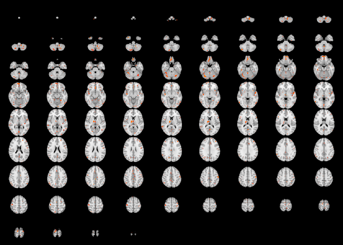
Figure 4.24: An example of a custom layout for the test of the age by sex interaction, with a CFT of \(p=0.01\).
4.3.4 Writing the results and viewing interactively
Papaya can be used to interactively visualize the statistical image.
To do this, we first have to write the results to a nifti image on the hard drive. The first two lines of code create a temporary directory to write the image.
We then use write.statMap function to write the image to disk.
The final line visualizes the statistical image overlayed on the template using Papaya.
We can use the qchisq function as above to threshold the statistical image.
# Visualize the chi square image
statmapFolder = tempfile() # generate a random file folder name
dir.create(statmapFolder) # create the directory
files = write.statMap(robustStatMap, outdir=statmapFolder) # write the statistical image
## Writing stat and coef images.## Writing sqrtSigma object.papaya(c(templatefile, files$stat )) # view the statistical image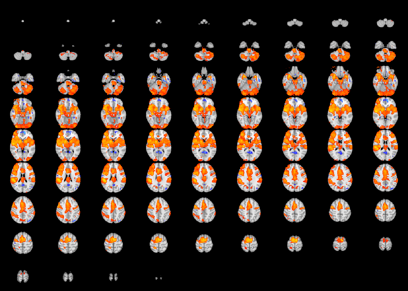
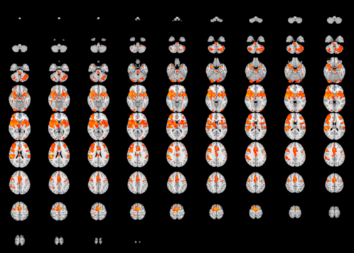
 We can create a summary table for the local maxima prior to running